Randomization, Contrasts,
and one-way ANOVA

STAT 6160 • Experimental Design • Fall 2026

Siddharth Vishwanath

Agenda

§1. Notation

§2. The completely randomized design

§3. Randomization

§4. One-way ANOVA

§5. Multiple comparisons

§6. Contrasts

§1. Notation

Indices

\[y_{ij} = \text{observation of unit $j$ on treatment $i$}, \\ i = 1,\ldots,g, \quad j = 1,\ldots,n_i\]

$g$ treatments
- (e.g., $g=3$ when we have placebo, treatment 1 and treatment 2)
$n_i$ units on each treatment $i$
- (e.g., $n_1$ units on placebo, $n_2$ units on treatment 1, and $n_3$ units on treatment 2)
The total number of experimental units is $\displaystyle N = \sum_{i=1}^{g} n_i$
Balanced means when:
- $n_1 = \cdots = n_g = n$, so $N = gn$

The dot convention

A dot replaces an index that has been averaged over.

\[ \bar y_{i\b} \ = \ \frac{1}{n_i}\sum_{j=1}^{n_i} y_{ij}, \qquad \bar y_{\b j} \ = \ \frac{1}{g}\sum_{i=1}^{g} y_{ij}, \qquad \bar y_{\b\b} \ = \ \frac{1}{N}\sum_{i=1}^{g}\sum_{j=1}^{n_i} y_{ij} \]

$\bar y_{i\b}$ : treatment mean
$\bar y_{\b j}$ : mean across treatments at position $j$ (defined when $n_i \equiv n$)
$\bar y_{\b\b}$ : grand mean

In the balanced case:
- $\displaystyle\bar y_{\b\b} = \frac{1}{g}\sum_i \bar y_{i\b}$;

in general:
- $\displaystyle\bar y_{\b\b} = \frac{1}{N}\sum_i n_i \bar y_{i\b}$

§2. The completely randomized design

The smallest experiment

Two treatments, $n_1$ and $n_2$ units.

\[ \begin{aligned} y_{ij} &= \mu + \tau_i + \e_{ij}, &\qquad \e_{ij} &\iid \mathcal{N}(0,\sigma^2) \\ &i = 1,2, & j &= 1,\ldots,n_i \end{aligned} \]

Target $\Delta \ = \ \E(y_{1j}) - \E(y_{2j}) \ = \ \tau_1 - \tau_2$
$\hat\Delta = \bar y_{1\b} - \bar y_{2\b}$, and $s_p^2$ pools the two within-group variances

\[ t \ = \ \frac{\hat\Delta - \Delta}{s_p\sqrt{1/n_1 + 1/n_2}} \ \sim \ t_{(n_1+n_2-2)} \]

The same test as a regression

\[ y_i \ = \ \beta_0 + \beta_1 w_i + \e_i, \qquad w_i = \begin{cases} 0 & \text{treatment 1} \\ 1 & \text{treatment 2}\end{cases} \]

\[ \Xv \ = \ \pc{\ \onev \ \ \ \wv \ }, \qquad \hat\beta_1 = \bar y_{2\b} - \bar y_{1\b}, \qquad \pa{(\Xv^\top\Xv)^{-1}}_{22} = \frac{1}{n_1} + \frac{1}{n_2} \]

$H_0 : \beta_1 = 0$ is the one-row general linear hypothesis $\cv^\top\betav = 0$
$\tau_2 - \tau_1$ is estimable; $\tau_1$ and $\tau_2$ separately are not

Why only the difference is identified

The two treatment means are

\[ \mu_1 = \mu + \tau_1, \qquad \mu_2 = \mu + \tau_2. \]

For any number $\eta$, shifting the parameters gives exactly the same two means:

\[ \mu + \tau_i = (\mu - \eta) + (\tau_i + \eta), \qquad i = 1,2. \]

Thus $\tau_1-\tau_2$ is unchanged, but neither $\tau_1$ nor $\tau_2$ has a unique value. The treatment-effects design matrix is

\[ \underbrace{ \begin{pmatrix} \onev_{n_1} & \onev_{n_1} & \zerov_{n_1} \\ \onev_{n_2} & \zerov_{n_2} & \onev_{n_2} \end{pmatrix} }_{\Xv_{\tau}\ \in\ \R^{N\times3},\quad \rank(\Xv_{\tau})=2} \qquad \begin{pmatrix}\mu\\\tau_1\\\tau_2\end{pmatrix}. \]

The shorthand $\Xv_{\tau} = [\onev\ \zv_1\ \zv_2]$ is convenient. Since

\[ \qquad \onev = \zv_1 + \zv_2, \]

the first column is already the sum of the other two.

With the usual reference-cell dummy encoding, instead drop the second column ($\zv_1$):

\[ \Xv_{\mathrm{ref}} = \pc{\ \onev\ \ \zv_2\ }, \qquad \beta_0 = \mu_1, \qquad \beta_1 = \mu_2 - \mu_1. \]

HW: Why?

Four assumptions

\[ (\text{A1 }) \e_i \sim \mathcal{N}(0,\sigma^2) \qquad (\text{A2 }) \var(\e_i) \text{ free of } w_i \qquad (\text{A3 }) \e_i \text{ independent} \\ (\text{A4 }) w_i \text{ is unrelated to omitted } u_i \]

($A1$): CLT limits the damage
($A2$): little damage when $n_1 = n_2$; otherwise Welch, $\sqrt{s_1^2/n_1 + s_2^2/n_2}$
($A3$): violations are hard to detect
($A4$) is a design risk, not a distributional assumption. Consider

\[ \E(y_i) = \beta_0 + \beta_1 w_i + \beta_2 u_i. \]

Leaving out $u_i$ is harmful when it is systematically associated with treatment. * Complete randomization makes that association average to zero over the randomization; it does not make $u_i$ disappear from an individual experiment

The design decision

$N$ units, $g$ treatments, group sizes $n_1,\ldots,n_g$ fixed in advance
The experimenter chooses the map from units to treatments, and nothing else
Completely randomized design: that map is drawn uniformly over all $\displaystyle \binom{N}{n_1,\ n_2,\ \ldots,\ n_g}$ allocations
Alternatives in use: systematic order, alternation, convenience order

§3. Randomization

Setup

Two thumbnail designs, A and B, on one account. Ten posting slots $i = 1,\ldots,10$, one per hour, five slots per design. Response $y_i$ is engagement in the hour after the post.

S1. Blocked

AAAAABBBBB

S2. Alternating

ABABABABAB

S3. Randomized

ABBBAABAAB

The error structure

\[ \hat\Delta - \Delta \ = \ \frac{1}{5}\sum_{i=1}^{10} v_i\,\e_i \]

\[ v_i \ = \ \begin{cases} +1 & \text{slot } i \text{ gets A}\\ -1 & \text{slot } i \text{ gets B} \end{cases} \]

S1. Blocked

AAAAABBBBB

\[ \frac{1}{5}\left(\sum_{i=1}^{5}\e_i - \sum_{i=6}^{10}\e_i\right) \]

S2. Alternating

ABABABABAB

\[ \frac{1}{5}\sum_{i=1}^{10}(-1)^{i+1}\e_i \]

S3. Randomized

ABBBAABAAB

\[ \frac{1}{5}\sum_{i=1}^{10}v_i\e_i \]

Bias from an omitted trend

Engagement drifts through the day: $u_i = c\,(i - 5.5)$, absorbed into $\e_i$.

\[ \E\big(\hat\Delta\big) - \Delta \ = \ \frac{c}{5}\sum_{i=1}^{10} v_i\,(i - 5.5) \]

AAAAABBBBB

\[ \sum_i v_i(i-5.5) = -25 \] \[ \text{bias} = -5c \]

ABABABABAB

\[ \sum_i v_i(i-5.5) = -5 \] \[ \text{bias} = -c \]

ABBBAABAAB

\[ \sum_i v_i(i-5.5) = 3 \] \[ \text{bias} = 0.6c \]

Alternation has its own blind spot

Suppose engagement alternates for an unrecorded reason: $u_i = c\,(-1)^i$. Then

\[ \E\big(\hat\Delta\big) - \Delta \ = \ \frac{c}{5}\sum_{i=1}^{10} v_i(-1)^i \]

Schedule	$\sum_i v_i(-1)^i$	Bias
S1: blocked	$0$	$0$
S2: alternating	$-10$	$-2c$
S3: randomized	$-2$	$-0.4c$

Randomization is not magic for one realized allocation. Its protection is that, over the draw, the bias is centered at zero for any fixed pattern $u_i$.

Variance under adjacent correlation

\[ \mathrm{corr}(y_i, y_{i'}) \ = \ \begin{cases} 1 & i = i'\\ \rho & |i - i'| = 1\\ 0 & \text{else} \end{cases} \qquad\Longrightarrow\qquad \var\big(\hat\Delta\big) \ = \ \frac{\sigma^2}{25}\pa{10 + 2\rho\sum_{i=1}^{9} v_i v_{i+1}} \]

AAAAABBBBB

\[ \textstyle\sum_i v_i v_{i+1} = 7 \] \[ \tfrac{2\sigma^2}{5} + \tfrac{14\rho\sigma^2}{25} \]

ABABABABAB

\[ \textstyle\sum_i v_i v_{i+1} = -9 \] \[ \tfrac{2\sigma^2}{5} - \tfrac{18\rho\sigma^2}{25} \]

ABBBAABAAB

\[ \textstyle\sum_i v_i v_{i+1} = -1 \] \[ \tfrac{2\sigma^2}{5} - \tfrac{2\rho\sigma^2}{25} \]

The reported standard error uses $\rho = 0$ in all three cases.

Drawing an allocation

Permute the unit labels, cut into groups of sizes $n_1,\ldots,n_g$
Assignment order and measurement order are separate randomizations
Restricted randomization: re-draw when the realized allocation is unbalanced on a known covariate
The realized allocation is part of the data

§4. One-way ANOVA

From two treatments to $g$

\[ \begin{aligned} y_{ij} &= \mu + \tau_i + \e_{ij}, &\qquad \e_{ij} &\iid \mathcal{N}(0,\sigma^2) \\ &i = 1,\ldots,g, & j &= 1,\ldots,n_i \end{aligned} \]

$g = 2$ gives §2, and $H_0 : \tau_1 = \tau_2$ is the two-sample $t$-test
$g > 2$: $H_0 : \tau_1 = \cdots = \tau_g$ is $g-1$ restrictions, not one
(Alternatively) Cell-mean form:

\[ y_{ij} = \mu_i + \e_{ij}, \qquad \mu_i = \mu + \tau_i \]

There are $g$ group means but $g+1$ symbols in $(\mu,\tau_1,\ldots,\tau_g)$.

Why one-way ANOVA needs a constraint

Let $\zv_i$ indicate membership in treatment $i$. The treatment-effects design matrix is

\[ \underbrace{ \begin{pmatrix} \onev_{n_1} & \onev_{n_1} & \zerov_{n_1} & \cdots & \zerov_{n_1} \\ \onev_{n_2} & \zerov_{n_2} & \onev_{n_2} & \cdots & \zerov_{n_2} \\ \vdots & \vdots & \vdots & \ddots & \vdots \\ \onev_{n_g} & \zerov_{n_g} & \zerov_{n_g} & \cdots & \onev_{n_g} \end{pmatrix} }_{\Xv_{\tau}\ \in\ \R^{N\times(g+1)},\quad \rank(\Xv_{\tau})=g} \qquad \begin{pmatrix}\mu\\\tau_1\\\tau_2\\\vdots\\\tau_g\end{pmatrix}. \]

The shorthand $\Xv_{\tau} = [\onev\ \zv_1\ \cdots\ \zv_g]$ is convenient. Since $\onev = \zv_1 + \zv_2 + \cdots + \zv_g$, it has $g+1$ columns but rank only $g$: one column is redundant. Equivalently, for every $\eta$,

\[ \mu + \tau_i = (\mu - \eta) + (\tau_i + \eta), \qquad i = 1,\ldots,g. \]

The fitted group means do not change. A constraint simply chooses one coordinate system for the same fitted values:

\[ \sum_i n_i\tau_i=0 \quad \text{(deviations from the weighted grand mean)}, \qquad \tau_1=0 \quad \text{(treatment 1 as reference)}, \]

or use the $g$ cell means directly and omit $\mu$.

With reference-cell dummy encoding, drop the second column ($\zv_1$):

\[ \Xv_{\mathrm{ref}} = \pc{\ \onev\ \ \zv_2\ \ \cdots\ \ \zv_g\ }, \qquad \gamma_0 = \mu_1, \qquad \gamma_{i-1} = \mu_i - \mu_1, \quad i = 2,\ldots,g. \]

The intercept is the treatment-1 mean; every other coefficient is that treatment’s difference from treatment 1. The fitted group means are unchanged.

Diet Restriction and Longevity

Does restricting food intake extend the lives of mice?

349 female mice were randomly assigned to six diets; the response is lifetime in months. (Weindruch et al. 1986; Ramsey and Schafer 2013)

Diet	What the mice received	$n_i$
A: (N/N85)	Normal before weaning; 85 kcal/week afterward	57
B: (NP)	Unlimited standard, nonpurified food	49
C: (N/R50)	Normal before weaning; 50 kcal/week afterward	71
D: (R/R50)	Restriction before and after weaning; 50 kcal/week afterward	56
E: (lopro)	As C, with protein reduced as mice aged	56
F: (N/R40)	Normal before weaning; 40 kcal/week afterward	60

We use A as the reference for comparisons of restricted regimens. B is a separate standard-diet benchmark.

Diet Restriction and Longevity: scatter plot

import pandas as pd
import numpy as np
import matplotlib.pyplot as plt

d = pd.read_csv("data/longevity.csv")
order = ["A", "B", "C", "D", "E", "F"]
colors = ["gray", "#0072B2", "#E69F00",
          "#009E73", "#CC79A7", "#D55E00"]
rng = np.random.default_rng(6160)

fig, ax = plt.subplots()
for i, (diet, color) in enumerate(zip(order, colors)):
    y = d.loc[d.Diet == diet, "Lifetime"]
    x = i + rng.uniform(-0.15, 0.15, len(y))
    ax.scatter(x, y, color=color, alpha=0.65)
ax.set(xticks=range(6), xticklabels=order,
       ylabel="Lifetime (months)")
fig.tight_layout()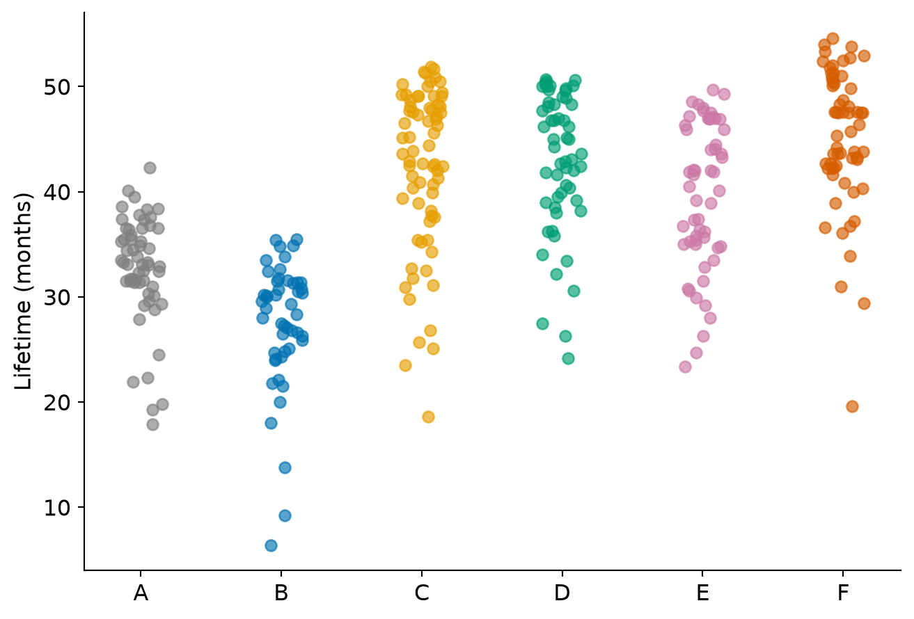

Individual mouse lifetimes across six diet groups, with substantial within-group spread and generally longer lives under restricted regimens. — Figure 1

Small horizontal offsets separate overlapping points within each diet.

Diet Restriction and Longevity: boxplot

groups = [
    d.loc[d.Diet == diet, "Lifetime"]
    for diet in order
]

fig, ax = plt.subplots()
boxes = ax.boxplot(
    groups, tick_labels=order,
    patch_artist=True
)
for box, color in zip(boxes["boxes"], colors):
    box.set_facecolor(color)
    box.set_alpha(0.65)
ax.set_ylabel("Lifetime (months)")
fig.tight_layout()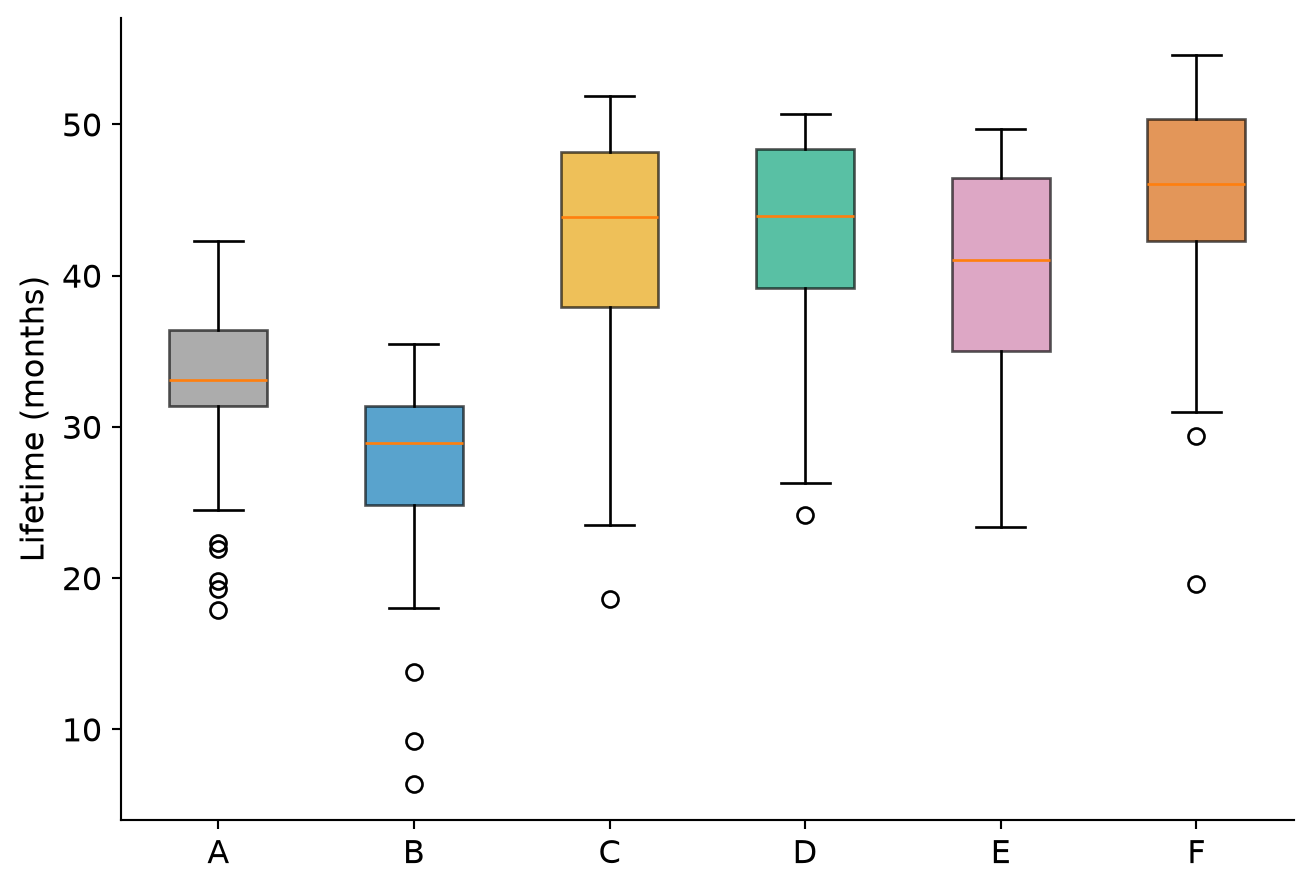

Boxplots of lifetimes by diet. The standard unrestricted diet has the lowest median; the 40 kcal diet has the highest. Several groups have low outliers. — Figure 2

Which differences look large relative to the spread within a diet?

Diet Restriction and Longevity: The model

For mouse $j$ receiving diet $i$, \[ y_{ij}=\mu_i+\e_{ij},\qquad \e_{ij}\iid\mathcal N(0,\sigma^2), \quad i=1,\ldots,6,\quad j=1,\ldots,n_i. \]

$\mu_i$: mean lifetime under diet $i$.
$\sigma$: within-diet standard deviation, assumed common to all six diets.
Equivalent treatment-effects form: $\mu_i=\mu+\tau_i$.

\[ H_0:\mu_1=\cdots=\mu_6 \qquad\text{versus}\qquad H_A:\text{at least one mean differs}. \] This tests equality of all six means, including the B group.

Diet Restriction and Longevity: The design matrix

Order the groups as A, B, C, D, E, F. With A as reference, the design matrix in block form is

\[ \Xv = \underbrace{ \begin{pmatrix} \onev_{57} & \zerov_{57} & \zerov_{57} & \zerov_{57} & \zerov_{57} & \zerov_{57} \\ \onev_{49} & \onev_{49} & \zerov_{49} & \zerov_{49} & \zerov_{49} & \zerov_{49} \\ \onev_{71} & \zerov_{71} & \onev_{71} & \zerov_{71} & \zerov_{71} & \zerov_{71} \\ \onev_{56} & \zerov_{56} & \zerov_{56} & \onev_{56} & \zerov_{56} & \zerov_{56} \\ \onev_{56} & \zerov_{56} & \zerov_{56} & \zerov_{56} & \onev_{56} & \zerov_{56} \\ \onev_{60} & \zerov_{60} & \zerov_{60} & \zerov_{60} & \zerov_{60} & \onev_{60} \end{pmatrix} }_{349\times6,\quad \rank(\Xv)=6}. \]

Here $\onev_n$ and $\zerov_n$ are $n\times1$ vectors of ones and zeros.

The intercept is $\mu_{\mathrm{A}}$; the other coefficients are $\mu_i-\mu_{\mathrm{A}}$. The fitted value for every mouse is its diet’s sample mean.

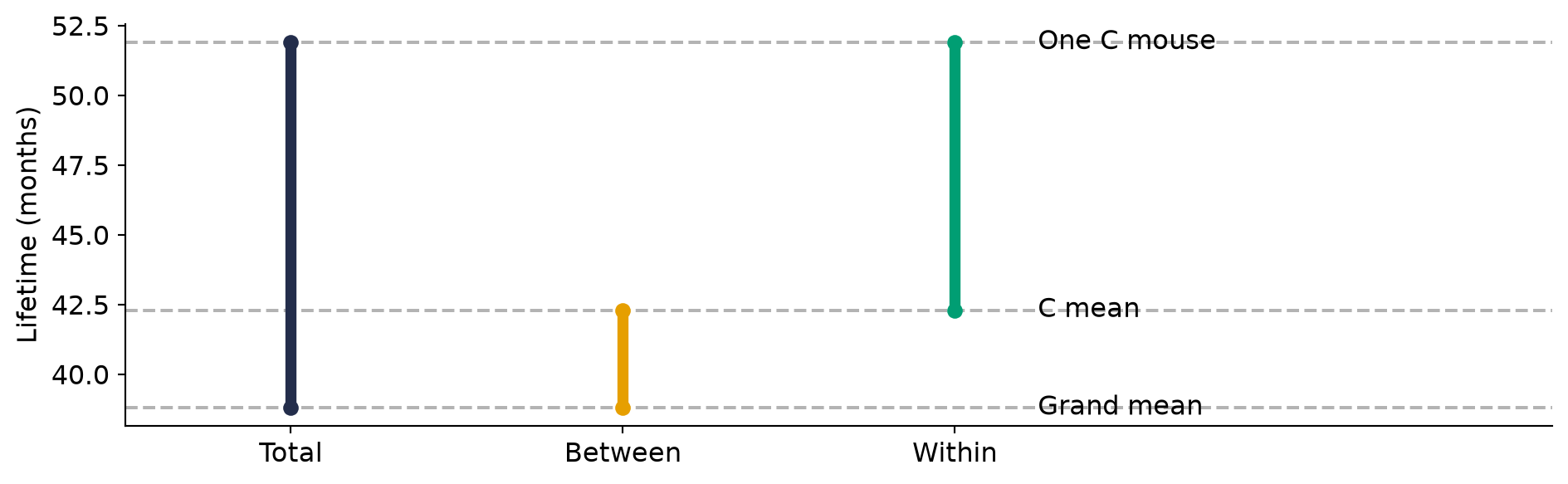
Between-diet and within-diet variation

\[ \underbrace{y_{ij}-\bar y_{\b\b}}_{\text{total deviation}} = \underbrace{\bar y_{i\b}-\bar y_{\b\b}}_{\text{between diets}} + \underbrace{y_{ij}-\bar y_{i\b}}_{\text{within diet}}. \]

A mouse's lifetime is compared with its diet mean and the grand mean. Segments show total, between-diet, and within-diet deviations. — Figure 3

From deviations to sums of squares

\[ \underbrace{\sum_{i,j}(y_{ij}-\bar y_{\b\b})^2}_{\sstot} = \underbrace{\sum_i n_i(\bar y_{i\b}-\bar y_{\b\b})^2}_{\sstrt} + \underbrace{\sum_{i,j}(y_{ij}-\bar y_{i\b})^2}_{\ssres}. \]

Between: how far the six diet means lie from the grand mean, weighted by group size.
Within: how much individual lifetimes vary around their own diet mean.

Why does the cross term vanish? \[ \sum_{i,j}(\bar y_{i\b}-\bar y_{\b\b})(y_{ij}-\bar y_{i\b}) =\sum_i(\bar y_{i\b}-\bar y_{\b\b}) \underbrace{\sum_j(y_{ij}-\bar y_{i\b})}_{0}=0. \]

The geometry and degrees of freedom

\[ \mathbb R^{349} = \underbrace{\mathrm{span}(\onev)}_{1} \oplus \underbrace{\bigl(\mathcal C(\Xv)\cap\onev^\perp\bigr)}_{5} \oplus \underbrace{\mathcal C(\Xv)^\perp}_{343}. \]

One grand mean.
Six fitted diet means minus one grand mean: $g-1=5$ between-diet degrees of freedom.
349 observations minus six fitted means: $N-g=343$ residual degrees of freedom.

The centered response has $348=5+343$ degrees of freedom. Orthogonal components give the sums-of-squares identity by Pythagoras.

The null distribution of the F statistic

Under $H_0$ and the normal, common-variance model, \[ \frac{\sstrt}{\sigma^2}\sim\chi^2_{5},\qquad \frac{\ssres}{\sigma^2}\sim\chi^2_{343}, \quad\text{independently}. \]

Therefore both mean squares estimate the same $\sigma^2$ under $H_0$: \[ F=\frac{\sstrt/5}{\ssres/343}\sim F_{5,343}. \]

When diet means differ, the expected treatment mean square increases: \[ \E(\mathrm{MS_{trt}})=\sigma^2+ \frac{\sum_i n_i(\mu_i-\mu_w)^2}{g-1}, \qquad \mu_w=\frac{\sum_i n_i\mu_i}{N}. \] Large values of $F$ provide evidence against equality of the diet means.

The ANOVA table

Source	df	Sum of squares	Mean square
Diet	$g-1=5$	$\sstrt$	$\sstrt/5$
Residual	$N-g=343$	$\ssres$	$\ssres/343$
Total	$N-1=348$	$\sstot$

\[ F=\frac{\mathrm{MS_{trt}}}{\mathrm{MS_{res}}}, \qquad \hat\sigma=\sqrt{\mathrm{MS_{res}}}, \qquad R^2=\frac{\sstrt}{\sstot}. \]

Unequal group sizes change the weights, not this decomposition.

Diet Restriction and Longevity: Linear model

import statsmodels.formula.api as smf

# First category becomes the reference.
d["Diet"] = pd.Categorical(
    d.Diet, categories=order
)
fit = smf.ols(
    "Lifetime ~ C(Diet)", data=d
).fit()

coef = pd.DataFrame({
    "Estimate": fit.params,
    "SE": fit.bse
})
coef.index = ["A mean"] + [
    diet + " - A" for diet in order[1:]
]
coef.round(2)

	Estimate	SE
A mean	32.69	0.88
B - A	-5.29	1.30
C - A	9.61	1.19
D - A	10.19	1.26
E - A	6.99	1.26
F - A	12.43	1.24

The intercept is a mean in months; every other estimate is a difference in months. These standard errors pool within-diet variation from all six groups.

Diet Restriction and Longevity: ANOVA Table

from statsmodels.stats.anova import anova_lm

anova = anova_lm(fit)
anova.round(3)

	df	sum_sq	mean_sq	F	PR(>F)
C(Diet)	5.0	12733.942	2546.788	57.104	0.0
Residual	343.0	15297.415	44.599	NaN	NaN

$F_{5,343}=57.10$, $p=4.11e-43$; $\hat\sigma=6.68$ months.

We have evidence that the six mean lifetimes are not all equal. Comparisons with A require tests of the individual mean differences.

Diet Restriction and Longevity: check the model

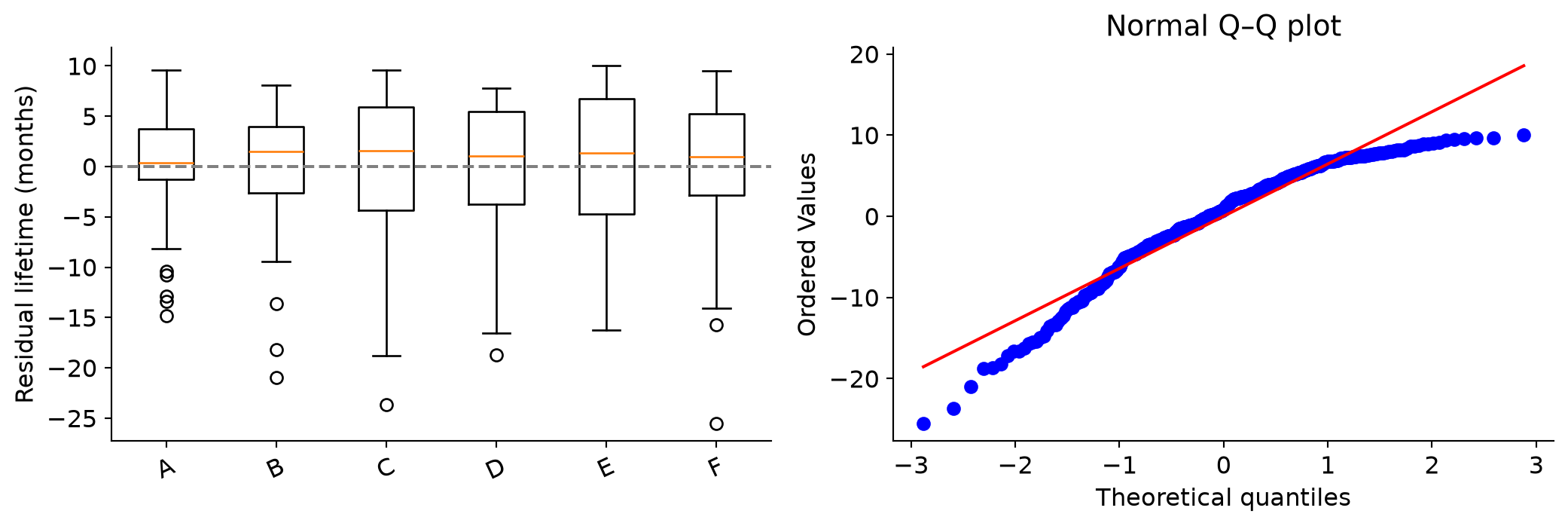
Residuals by diet and normal quantile plot assess common variance and normality; low lifetime observations produce a lower-tail departure. — Figure 4

The plots show differences in spread and departures from normality in the lower tail.
Assessing independence requires information about housing and how the experiment was run.
Welch’s ANOVA allows unequal variances; subsequent contrasts also need standard errors that allow unequal variances.

Comparing C and A: 50 and 85 kcal/week

Does reducing the ration from 85 to 50 kcal/week after weaning change mean lifetime?

Groups C and A both received normal feeding before weaning: \[ \theta=\mu_{\mathrm{C}}-\mu_{\mathrm{A}}. \]

In our six-diet order, the coefficients are \[ \cv=(-1,\ 0,\ 1,\ 0,\ 0,\ 0). \] The unrestricted B group is not part of this particular comparison.

Contrasts among diet means

\[ \theta=\sum_i c_i\mu_i,\qquad \sum_i c_i=0. \]

Question	Coefficients in our diet order
C versus A: 50 versus 85 kcal after weaning	$(-1,0,1,0,0,0)$
D versus C: earlier versus later restriction at 50 kcal	$(0,0,-1,1,0,0)$
F versus C: 40 versus 50 kcal after weaning	$(0,0,-1,0,0,1)$
E versus C: reduced protein	$(0,0,-1,0,1,0)$

Because the coefficients sum to zero, $\sum_i c_i\mu_i=\sum_i c_i\tau_i$: the answer is unchanged by the identifiability constraint.

Inference for one contrast

\[ \hat\theta=\sum_i c_i\bar y_{i\b},\qquad \mathrm{se}(\hat\theta)= \sqrt{\mathrm{MS_{res}}\sum_i\frac{c_i^2}{n_i}}. \]

Under $H_0:\theta=\theta_0$, \[ t=\frac{\hat\theta-\theta_0}{\mathrm{se}(\hat\theta)} \sim t_{343}. \]

A pointwise 95% confidence interval is \[ \hat\theta\pm t_{343}^{0.975}\mathrm{se}(\hat\theta). \]

For C versus A (50 versus 85 kcal), only $1/71+1/57$ enters the variance multiplier.

Diet Restriction and Longevity: one contrast

# Coefficients here refer to regression
# parameters: intercept, then differences.
test = fit.t_test([0, 0, 1, 0, 0, 0])
test.summary_frame().T.round(3)

	c0
coef	9.606
std err	1.188
t	8.088
P>\|t\|	0.000
Conf. Int. Low	7.270
Conf. Int. Upp.	11.942

Estimated change: 9.61 months; pointwise 95% CI: (7.27, 11.94) months.

Why does the coefficient vector in the Python call differ from $\cv$?

Comparing C–F with A

How does the average of groups C–F (the four restricted regimens) compare with A?

\[ \cv=(-1,0,\tfrac14,\tfrac14,\tfrac14,\tfrac14). \]

This gives each regimen equal weight, despite unequal sample sizes. Pooling all restricted mice would give a different, sample-size-weighted estimand.

Contrasts and the ANOVA decomposition

For a null contrast $\theta=0$, \[ \mathrm{SS}(\cv)=\frac{\hat\theta^2}{\sum_i c_i^2/n_i}, \qquad F_{\text{one contrast}}=\frac{\mathrm{SS}(\cv)}{\mathrm{MS_{res}}}=t^2. \]

Two estimated contrasts are uncorrelated precisely when \[ \sum_i\frac{c_i c_i'}{n_i}=0. \]

Five mutually orthogonal contrasts partition the diet SS into five 1-df pieces.
Non-orthogonal contrasts can be estimated and tested, but their sums of squares generally do not partition the diet SS.

C versus A and F versus A share the same reference mean. Their covariance is $\sigma^2/57>0$: their sums of squares do not simply add.

Scheffé’s test for a contrast

For $H_0:\theta=\sum_i c_i\mu_i=0$, with $\sum_i c_i=0$, write \[ t_{\cv}=\frac{\hat\theta} {\sqrt{\mathrm{MS_{res}}\sum_i c_i^2/n_i}}. \]

Scheffé’s method rejects $H_0$ when \[ |t_{\cv}|>\sqrt{(g-1)F_{g-1,N-g}^{1-\alpha}}, \qquad\text{equivalently}\qquad \frac{t_{\cv}^2}{g-1}>F_{g-1,N-g}^{1-\alpha}. \]

This controls the probability of any false rejection across all contrasts at level $\alpha$, under the normal, common-variance model. It therefore also covers contrasts selected after examining the data.

Scheffé confidence intervals

Simultaneous $100(1-\alpha)\%$ intervals for all contrasts are \[ \hat\theta\ \pm\ \underbrace{\sqrt{(g-1)F_{g-1,N-g}^{1-\alpha}}}_{\text{Scheffé multiplier}} \sqrt{\mathrm{MS_{res}}\sum_i\frac{c_i^2}{n_i}}. \]

For the six diets, the multiplier is $\sqrt{5F_{5,343}^{0.95}}$.

These intervals are wider than pointwise $t$ intervals because they cover all contrasts simultaneously. For comparisons only with A, Dunnett’s method gives narrower intervals.

Diet Restriction and Longevity: Scheffé test

Compare the average of groups C–F (the restricted diets) with A: \[ \theta=\frac{\mu_{\mathrm{C}}+\mu_{\mathrm{D}} +\mu_{\mathrm{E}}+\mu_{\mathrm{F}}}{4} -\mu_{\mathrm{A}}. \]

# Weights on the reference-coded parameters.
result = fit.t_test([0, 0, .25, .25, .25, .25])
effect = result.effect.item()
se = result.sd.item()
df = fit.df_resid
k = len(order) - 1
critical = np.sqrt(k * stats.f.ppf(.95, k, df))
p_scheffe = stats.f.sf((effect / se)**2 / k, k, df)

pd.Series({
    "Estimate (months)": effect,
    "SE (months)": se,
    "Scheffe lower": effect - critical * se,
    "Scheffe upper": effect + critical * se,
    "Adjusted p": p_scheffe
}).to_frame("Value")

	Value
Estimate (months)	9.805092e+00
SE (months)	9.837196e-01
Scheffe lower	6.512712e+00
Scheffe upper	1.309747e+01
Adjusted p	2.122759e-17

Multiple comparisons and Type I error

We test groups B–F against A. Together, these tests form a family of comparisons.

\[ \mathrm{FWER}=\Pr(\text{at least one false rejection in the family}). \]

Five independent level-0.05 tests would give $1-0.95^5\approx0.226$.
Our tests are dependent, because each uses the same reference group.
The adjustment covers all five comparisons, including those we do not report.

Rejecting the omnibus null does not control the familywise error rate of unadjusted follow-up tests. Dunnett’s procedure controls this rate without a preliminary omnibus test.

Multiple-comparison procedures

Comparisons included	Procedure	Scope of simultaneous inference
Groups B–F versus A	Dunnett	All five reference comparisons
All 15 pairwise diet differences	Tukey–Kramer	All pairs, allowing unequal $n_i$
$K$ contrasts specified before examining the data	Bonferroni	All $K$ contrasts
Any contrast, including one selected after seeing data	Scheffé	The entire contrast family

Bonferroni uses $t_{343}^{1-\alpha/(2K)}$ for two-sided intervals; Scheffé uses $\sqrt{5F_{5,343}^{1-\alpha}}$.

Diet Restriction and Longevity: Dunnett comparisons

from scipy import stats

control = groups[0]  # A
dunnett = stats.dunnett(
    *groups[1:], control=control,
    alternative="two-sided",
    rng=np.random.default_rng(6160)
)
ci = dunnett.confidence_interval()
comparison = pd.DataFrame({
    "Difference": [
        y.mean() - control.mean()
        for y in groups[1:]
    ],
    "Lower": ci.low,
    "Upper": ci.high,
    "Adjusted p": dunnett.pvalue
}, index=order[1:])
comparison.round(3)

	Difference	Lower	Upper
B	-5.289	-8.572	-2.007
C	9.606	6.609	12.602
D	10.194	7.024	13.365
E	6.994	3.824	10.165
F	12.425	9.309	15.542

Intervals have joint 95% coverage under the common-variance normal model. Positive differences mean longer average life than A.

Diet Restriction and Longevity: simultaneous intervals

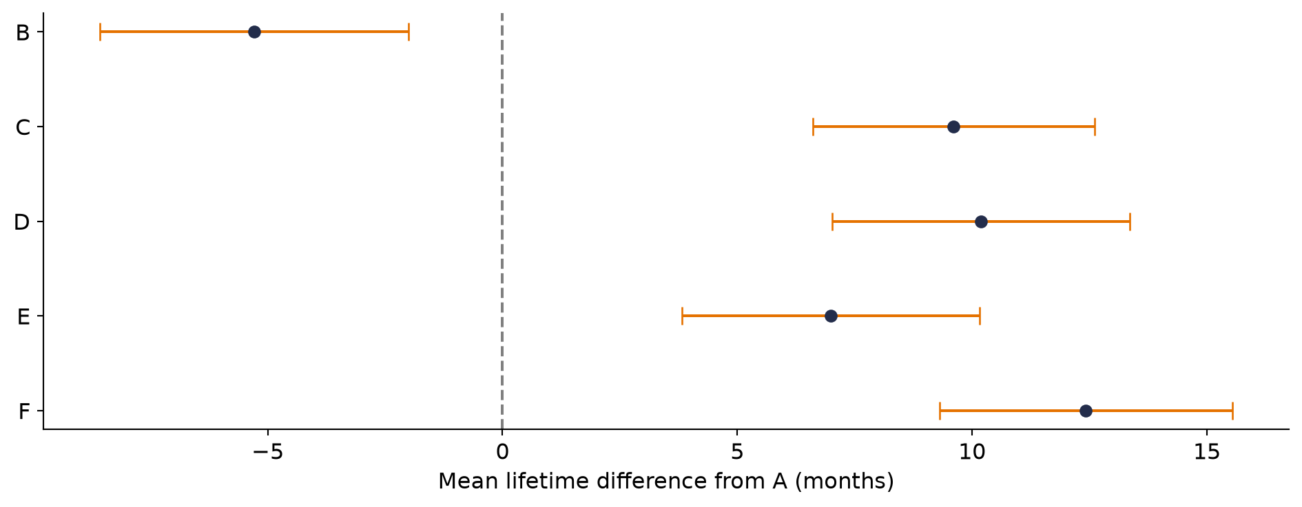
Simultaneous 95 percent Dunnett intervals for each diet minus A, with a vertical zero reference line. — Figure 5

Which diets have longer mean lifetimes than A, and by how many months? An interval containing zero is not evidence that the two diets are equivalent.

Summary

ANOVA: the data provide evidence against equality of the six diet means.
C versus A (50 versus 85 kcal/week): the estimated mean difference is 9.61 months.
Dunnett intervals: groups C–F have higher mean lifetimes than A; B has a lower mean.

These estimates apply to the mouse population and feeding conditions studied.

For next time

What if mice differed systematically by litter, cage, or experimental batch?
Pairing and blocking can account for known sources of variation.
Including these sources of variation can reduce the residual variance.

References

Ramsey, Fred L., and Daniel W. Schafer. 2013. The Statistical Sleuth: A Course in Methods of Data Analysis. 3rd ed. Cengage Learning.

Weindruch, Richard, Roy L. Walford, Suzanne Fligiel, and Donald Guthrie. 1986. “The Retardation of Aging in Mice by Dietary Restriction: Longevity, Cancer, Immunity and Lifetime Energy Intake.” The Journal of Nutrition 116 (4): 641–54. https://doi.org/10.1093/jn/116.4.641.

Schedule	\(\sum_i v_i(-1)^i\)	Bias
S1: blocked	\(0\)	\(0\)
S2: alternating	\(-10\)	\(-2c\)
S3: randomized	\(-2\)	\(-0.4c\)

Source	df	Sum of squares	Mean square
Diet	\(g-1=5\)	\(\sstrt\)	\(\sstrt/5\)
Residual	\(N-g=343\)	\(\ssres\)	\(\ssres/343\)
Total	\(N-1=348\)	\(\sstot\)

Question	Coefficients in our diet order
C versus A: 50 versus 85 kcal after weaning	\((-1,0,1,0,0,0)\)
D versus C: earlier versus later restriction at 50 kcal	\((0,0,-1,1,0,0)\)
F versus C: 40 versus 50 kcal after weaning	\((0,0,-1,0,0,1)\)
E versus C: reduced protein	\((0,0,-1,0,1,0)\)

Randomization, Contrasts, and one-way ANOVA

Agenda

§1. Notation

Indices

The dot convention

§2. The completely randomized design

The smallest experiment

The same test as a regression

Why only the difference is identified

Four assumptions

The design decision

§3. Randomization

Setup

The error structure

Bias from an omitted trend

Alternation has its own blind spot

Variance under adjacent correlation

Drawing an allocation

§4. One-way ANOVA

From two treatments to \(g\)

Why one-way ANOVA needs a constraint

Diet Restriction and Longevity

Diet Restriction and Longevity: scatter plot

Diet Restriction and Longevity: boxplot

Diet Restriction and Longevity: The model

Diet Restriction and Longevity: The design matrix

Between-diet and within-diet variation

From deviations to sums of squares

The geometry and degrees of freedom

The null distribution of the F statistic

The ANOVA table

Diet Restriction and Longevity: Linear model

Diet Restriction and Longevity: ANOVA Table

Diet Restriction and Longevity: check the model

Comparing C and A: 50 and 85 kcal/week

Contrasts among diet means

Inference for one contrast

Diet Restriction and Longevity: one contrast

Comparing C–F with A

Contrasts and the ANOVA decomposition

Scheffé’s test for a contrast

Scheffé confidence intervals

Diet Restriction and Longevity: Scheffé test

Multiple comparisons and Type I error

Multiple-comparison procedures

Diet Restriction and Longevity: Dunnett comparisons

Diet Restriction and Longevity: simultaneous intervals

Summary

For next time

References

Randomization, Contrasts,
and one-way ANOVA