Introduction

STAT 6160 • Experimental Design • Fall 2026

Siddharth Vishwanath

2026-08-25

\[ \newcommand{\pa}[1]{\left(#1\right)} \newcommand{\pb}[1]{\left\{#1\right\}} \newcommand{\pc}[1]{\left[#1\right]} \newcommand{\pA}[1]{\Big(#1\Big)} \newcommand{\pB}[1]{\Big\{#1\Big\}} \newcommand{\pC}[1]{\Big[#1\Big]} \newcommand{\eq}[1]{\begin{align}{#1}\end{align}} \newcommand{\eref}[1]{Eq.~\eqref{#1}} \newcommand{\pref}[1]{part~(\ref{#1})} \newcommand{\nn}{\nonumber} \newcommand{\n}{\nonumber\\} \newcommand{\f}{\frac} \newcommand{\defeq}{\stackrel{\small\bullet}{=}} \newcommand{\ra}{\rangle} \newcommand{\la}{\langle} \newcommand{\norm}[1]{\left\|#1\right\|} \newcommand{\abs}[1]{\left\lvert#1\right\rvert} \newcommand{\Abs}[1]{\Bigl\lvert#1\Bigr\rvert} \newcommand{\pr}{{\mathbb P}} \newcommand{\qr}{{\mathbb Q}} \newcommand{\xv}{{\boldsymbol{x}}} \newcommand{\av}{{\boldsymbol{a}}} \newcommand{\bv}{{\boldsymbol{b}}} \newcommand{\cv}{{\boldsymbol{c}}} \newcommand{\dv}{{\boldsymbol{d}}} \newcommand{\ev}{{\boldsymbol{e}}} \newcommand{\fv}{{\boldsymbol{f}}} \newcommand{\gv}{{\boldsymbol{g}}} \newcommand{\hv}{{\boldsymbol{h}}} \newcommand{\nv}{{\boldsymbol{n}}} \newcommand{\sv}{{\boldsymbol{s}}} \newcommand{\tv}{{\boldsymbol{t}}} \newcommand{\uv}{{\boldsymbol{u}}} \newcommand{\vv}{{\boldsymbol{v}}} \newcommand{\wv}{{\boldsymbol{w}}} \newcommand{\zerov}{{\mathbf{0}}} \newcommand{\onev}{{\mathbf{1}}} \newcommand{\phiv}{{\boldsymbol{\phi}}} \newcommand{\cc}{{\check{C}}} \newcommand{\xv}{{\boldsymbol{x}}} \newcommand{\Xv}{{\boldsymbol{X}\!}} \newcommand{\yv}{{\boldsymbol{y}}} \newcommand{\Yv}{{\boldsymbol{Y}}} \newcommand{\zv}{{\boldsymbol{z}}} \newcommand{\Zv}{{\boldsymbol{Z}}} \newcommand{\Iv}{{\boldsymbol{I}}} \newcommand{\Jv}{{\boldsymbol{J}}} \newcommand{\Cv}{{\boldsymbol{C}}} \newcommand{\Ev}{{\boldsymbol{E}}} \newcommand{\Fv}{{\boldsymbol{F}}} \newcommand{\Gv}{{\boldsymbol{G}}} \newcommand{\Hv}{{\boldsymbol{H}}} \newcommand{\alphav}{{\boldsymbol{\alpha}}} \newcommand{\epsilonv}{{\boldsymbol{\epsilon}}} \newcommand{\betav}{{\boldsymbol{\beta}}} \newcommand{\deltav}{{\boldsymbol{\delta}}} \newcommand{\gammav}{{\boldsymbol{\gamma}}} \newcommand{\etav}{{\boldsymbol{\eta}}} \newcommand{\piv}{{\boldsymbol{\pi}}} \newcommand{\thetav}{{\boldsymbol{\theta}}} \newcommand{\tauv}{{\boldsymbol{\tau}}} \newcommand{\muv}{{\boldsymbol{\mu}}} \newcommand{\argmin}{\mathop{\text{arg}\ \!\text{min}}} \newcommand{\arginf}{\mathop{\text{arg}\ \!\text{inf}}} \newcommand{\argmax}{\mathop{\text{arg}\ \!\text{max}}} \newcommand{\argsup}{\mathop{\text{arg}\ \!\text{sup}}} \newcommand{\f}{\frac} \newcommand{\e}{\epsilon} \newcommand{\b}{\bullet} \newcommand{\inv}{^{-1}} \newcommand{\A}{{\mathcal A}} \newcommand{\C}{{\mathbb C}} \newcommand{\E}{{\mathbb E}} \newcommand{\F}{{\mathcal{F}}} \newcommand{\N}{{\mathbb N}} \newcommand{\R}{{\mathbb R}} \newcommand{\Q}{{\mathbb Q}} \newcommand{\Z}{{\mathbb Z}} \newcommand{\X}{{\mathbb{X}}} \newcommand{\Y}{{\mathbb{Y}}} \newcommand{\G}{{\mathcal{G}}} \newcommand{\M}{{\mathcal{M}}} \newcommand{\Xn}{X_1, \dots, X_n} \newcommand{\Xm}{X_1, \dots, X_m} \newcommand{\Yn}{Y_1, \dots, Y_n} \newcommand{\Ym}{Y_1, \dots, Y_m} \newcommand{\Xb}{{\mathbb{X}}} \newcommand{\Yb}{{\mathbb{Y}}} \newcommand{\s}{{{\sigma}}} %%%%%%%%%%%%%%%%%%%%%%%%%%% \newcommand{\c}{^c} \newcommand{\bar}{\overline} \newcommand{\indep}{\perp\kern-6pt \perp} \newcommand{\pr}{{\mathbb P}} \newcommand{\R}{{\mathbb R}} \newcommand{\E}{{\mathbb E}} \newcommand{\var}{\text{Var}} \newcommand{\sd}{\text{SD}} \newcommand{\se}{\text{SE}} \newcommand{\ssres}{{\mathrm{SS}_{\mathrm{Res}}}} \newcommand{\sstrt}{{\mathrm{SS}_{\mathrm{Trt}}}} \newcommand{\sstot}{{\mathrm{SS}_{\mathrm{Tot}}}} \newcommand{\rank}{\mathop{\mathrm{rank}}} \newcommand{\supp}{\text{supp}} \newcommand{\Unif}{{\text{Unif}}} \newcommand{\Ber}{{\text{Ber}}} \newcommand{\Bin}{{\text{Bin}}} \newcommand{\Geo}{{\text{Geo}}} \newcommand{\Poi}{{\text{Poi}}} \newcommand{\Exp}{{\text{Exp}}} \newcommand{\Chisq}{{\chi^2}} \newcommand{\iid}{{\stackrel{iid}{\sim}}} \newcommand{\px}{p_{X}} \newcommand{\py}{p_{Y}} \newcommand{\pxy}{p_{X,Y}} \newcommand{\fx}{f_{X}} \newcommand{\fz}{f_{Z}} \newcommand{\fy}{f_{Y}} \newcommand{\fxy}{f_{X,Y}} \newcommand{\Fx}{F_{X}} \newcommand{\Fz}{F_{Z}} \newcommand{\Fy}{F_{Y}} \newcommand{\Fxy}{F_{X,Y}} \newcommand{\Xbar}{\overline{X}} \newcommand{\Ybar}{\overline{Y}} \newcommand{\Zbar}{\overline{Z}} \newcommand{\nXbar}{n \cdot \overline{X}} \newcommand{\nYbar}{n \cdot \overline{Y}} \newcommand{\nZbar}{n \cdot \overline{Z}} \newcommand{\Xn}{X_1, X_2, \dots, X_n} \newcommand{\Xm}{X_1, X_2, \dots, X_m} \newcommand{\Ym}{Y_1, Y_2, \dots, Y_m} \newcommand{\sumXn}{X_1 + X_2 + \dots + X_n} \newcommand{\la}{\ell_\alpha} \newcommand{\ua}{u_\alpha} \newcommand{\at}{{\alpha/2}} %%\renewcommand{\hat}{\widehat} \newcommand{\mux}{\mu_{X}} \newcommand{\muy}{\mu_{Y}} \newcommand{\sx}{\sigma_{X}} \newcommand{\sy}{\sigma_{Y}} \newcommand{\pvalue}{$p$-value} \newcommand{\Ho}{H_{0}} \newcommand{\Ha}{H_{a}} \]

Lecture slides sidv23.github.io/stat-6160

[0:00 — 1 min] Let the QR sit while people settle. Name, course number, and one line on where today is going: “one experiment from 1935, because most of what this course teaches is already in it.” Logistics later — they land better once people care.

To consult the statistician after an experiment is finished
is often merely to ask him to conduct a post mortem examination.

He can perhaps say what the experiment died of.

R. A. Fisher, 1938 (Fisher 1938)

[3:30 — 1.5 min] Read the top. Pause. Read the orange line. Don’t explain it.

Then: “Fisher wrote that in 1938. To see where it came from, back up a century.”

Before Fisher

Three things that came first

1809 · Least squares, and the normal curve
Gauss and Laplace, fitting orbits to noisy measurements. How to draw a line through error, and why error piles up in a bell shape. (Gauss 1809)

1889 · Correlation and regression
Galton, then Karl Pearson. Variation stops being a nuisance and becomes the thing you study. (Galton 1889)

1908 · Small samples
Gosset, a brewer at Guinness, publishing as “Student”. Exact answers from a dozen observations, because barley trials don’t give you thousands. (Student 1908)

All three: what to do with data you already have.

[5:00 — 2.5 min] Three beats, roughly 30 seconds each. Don’t teach any of them — this is scene-setting, and all three come back properly later in the term.

Gosset is the one worth lingering on. A working brewer, real experiments, tiny samples, and a boss who wouldn’t let him publish under his own name. He and Fisher corresponded for years. Barley connects Guinness to agriculture and agriculture to Rothamsted, which is where we’re going.

The fragment is the setup for the whole lecture: every one of these takes the data as given. Fisher asked the other question.

A lady tasting tea

Rothamsted, early 1920s

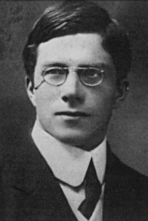
Fisher
statistician, in his 30s

Muriel Bristol
phycologist — she studied algae

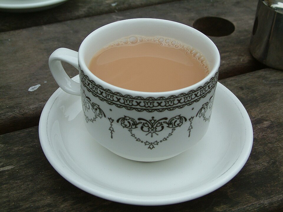
The tea
milk in first, or after

She turns down a cup. The milk went in after the tea, and she says she can tell.

The room laughs. Fisher asks the useful question: how would we find out?

[9:30 — 2.5 min] Tell it as a story. Keep three details: Rothamsted is an agricultural station, not a maths department; Bristol was a working scientist, not a party guest; and laughing is the normal response.

Use the missing photograph. It is not a gap, it’s the best twenty seconds on the slide: the most retold anecdote in statistics, and we don’t have a picture of the person at the centre of it, and the picture people did publish was the wrong woman. Good moment to say the story is partly legend — Salsburg’s retelling (Salsburg 2001) comes secondhand from someone who was there, and Senn (Senn 2012) has gone through what can actually be documented.

The pivot: Fisher takes neither side. He doesn’t argue about whether she can. He asks what evidence would settle it.

The design

Eight cups. Four milk-first, four tea-first.

Random order, fixed by the experimenter before she tastes anything.

She’s told the split — four of each — and names the four milk-first cups.

If she’s guessing

Her four picks have nothing to do with the truth. So every way of choosing four cups from eight is equally likely:

\[ \binom{8}{4} = 70 \]

All four right? One outcome out of 70. \(\;p = 1/70 \approx 0.014\).

[12:00 — 2.5 min] Slow down on “she’s told the split” — students skate past it, and it’s load-bearing. It’s what makes the reference set exactly 70 instead of something that depends on her guessing habits.

Build the 70 with them. Ask the room how many ways to pick four from eight; someone will say it.

Then the line: the 70 was known before she tasted anything. The design fixed the reference set in advance; the data only says where in it you landed.

Hold the null distribution — that’s the next slide.

Two designs

Design A

Fix four and four. Tell her the split. She names four.

\(\binom{8}{4} = 70\) ways.

Design B

Randomize each cup on its own, milk-first with probability \(1/2\). She judges each cup separately.

\(2^8 = 256\) ways.

Which would you rather run?

[14:30 — 1.5 min] Set it up, then take a show of hands on both. Don’t reveal anything.

Most rooms split, and a good number pick B — “independent” sounds more rigorous. That’s the misconception the widget takes apart, so it helps to have them commit out loud first.

Design A

she gets right

Design B

she gets right

[16:00 — 5 min] The centre of the lecture. Drive it; don’t narrate every number.

1. As it opens — both at a perfect score. A gives \(1/70 = 0.0143\), B gives \(1/256 = 0.0039\). Ask: “so B is better? It found more evidence.” Let it sit.
2. Drag A down to 3. Jumps to \(17/70 \approx 0.243\). One mistake wipes it out. That’s sensitivity — eight cups is a small experiment — and your first hook for power later in the term.
3. Press “deal 20 under B”. Use this, not repeated reshuffles: a single draw is badly lopsided only about 7% of the time, so clicking and hoping will strand you. Twenty reliably shows around six draws at 6–2 or worse. Point at one: “legal outcome, correctly randomized, and one tea cup in it.” Reshuffle is still good earlier — press it two or three times on A to show the split never moves.
4. Land it. B looked stronger because \(2^8 > \binom{8}{4}\) — a bigger reference set makes perfection rarer. That same freedom is what lets it hand you a useless experiment. A gives up some nominal significance and buys balance you don’t have to hope for.

If someone asks whether B can be fixed by conditioning on the realized split — yes, and it’s a good question. Conditioning on the margin takes you back to the hypergeometric. That’s Fisher’s exact test; we do it properly in a few weeks.

What’s actually new

• The null hypothesis is about the randomization, not a parameter of an assumed distribution. No normality, no large samples, no approximation

• The probability comes from something the experimenter physically did. Fisher didn’t assume a model of the world — he made one by shuffling cups

• So the \(p\)-value is exact, for a reason you can point at

• And the design came first

The null hypothesis is never proved or established, but is possibly disproved, in the course of experimentation.
— Fisher, 1935

[23:00 — 2.5 min] Most important slide in the lecture. Bullets two and three are the whole thing.

The line to hammer: randomization isn’t a hygiene rule, it’s what manufactures the distribution you compute against. Most students arrive thinking of it as a fairness ritual — something scrupulous people do. Reframe it as the source of the inference. If they leave with one idea, this is it.

Read the quote if you have time, skip it if not. It comes back when we do power.

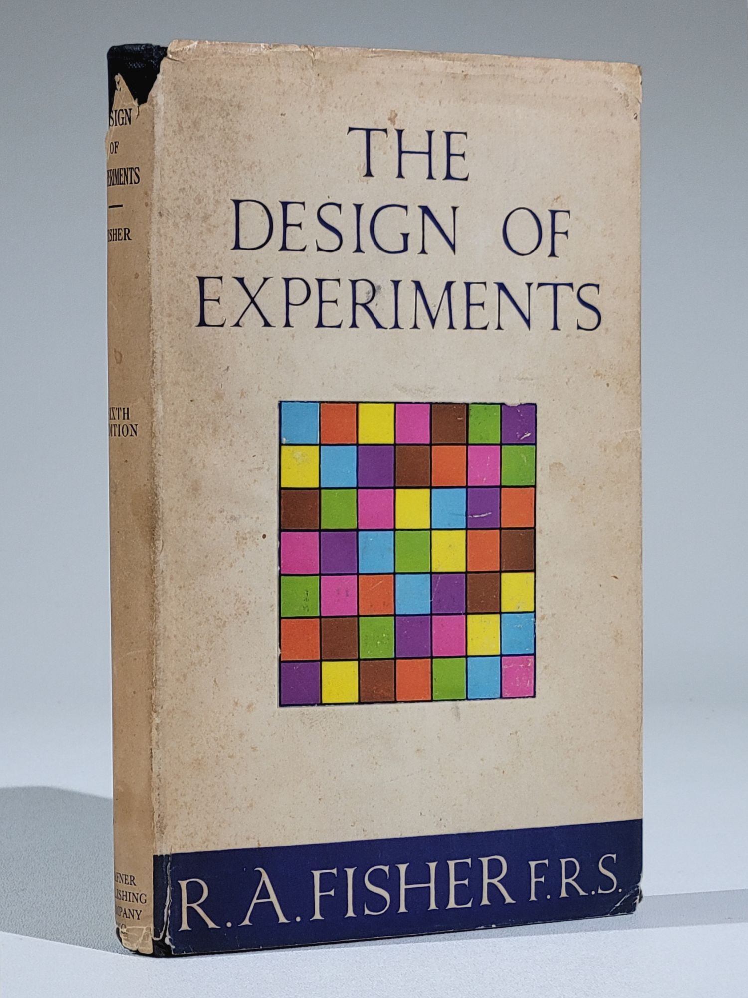
Ten years earlier: Statistical Methods for Research Workers (1925), which put these tools in the hands of people who weren’t statisticians (Fisher 1925). Every idea in the book was worked out for agriculture. All of them are now used to run experiments at companies that didn’t exist twenty years ago.

[25:30 — 1.5 min] Note for you, not the room: that book cover is a typographic mock-up I made, not a photograph. The 1935 Oliver & Boyd cover is still in copyright and there’s no free scan. If you own a copy, photograph it and drop it in at ../images/ — it’ll look better than my version.

Content: the striking thing is that a book about agricultural field trials opens with a party trick, and that the trick carries most of the theory.

The portability point is the one to land — these methods were built against a genuinely hostile problem, which is why they travel.

The other side

Fisher and tobacco

Fisher, 1952

1950s: Doll and Hill link smoking to lung cancer. In 1957 the Medical Research Council calls it cause and effect (Doll and Hill 1954).

Fisher disagrees, loudly. Letters to the BMJ in 1957, then a book in 1959 (Fisher 1959).

His argument: nobody randomized anything. The correlation is real, but some genetic factor could cause both the urge to smoke and the cancer.

He was also a paid consultant to the Tobacco Manufacturers’ Standing Committee, which funded the genetic work.

He was a pipe smoker.

He was wrong (Stolley 1991).

[27:00 — 2 min] Play it straight. No outrage, no defending him — the facts carry it.

The uncomfortable part, and the reason it’s in this lecture: his methodological point was correct. Observational data can’t rule out confounding, and nobody had randomized smoking. He was applying exactly the standard this course teaches, and he reached the wrong conclusion and took money from people with an interest in that conclusion.

Don’t resolve it here. Next slide.

Double-edged

• The same rigour that stops you believing too easily can be used to manufacture doubt

• Some things can’t be randomized. That doesn’t mean nothing can be known about them

• Being rigorous and being right are not the same thing

• Who pays you shapes what you’re willing to doubt

[29:00 — 2 min] Let this one breathe; it’s the slide people remember.

If the room is game, the question to leave open: what would have settled it? Answers worth surfacing — dose-response, mechanism, the fact that risk falls when people quit, animal work, consistency across many populations. That’s roughly the Bradford Hill argument, and it’s how causal knowledge gets built when randomization is off the table. We come back to it when we do observational designs.

Don’t moralize. Ask, then move.

Now

Where it shows up

Tech

A/B tests, interleaving, switchback designs, marketplaces where units interfere

Medicine

adaptive and platform trials, interim monitoring, dose-finding

Industry

response surfaces, robust design, process optimization

Machine learning

hyperparameter search, benchmark design, active learning, evals

Policy

field experiments, stepped-wedge rollouts

Science

computer experiments, self-driving labs, screening

Same question, bigger budget: what should we do next?

[31:00 — 1.5 min] Don’t read it. Point at two or three cells and move — this slide is peripheral vision.

Pick the column that matches the room. Ask early in the term what people work on and reuse this slide accordingly.

Then: “three of these break something we assumed today.”

Bandits

Fisher fixes the assignment before any data arrives. But if one treatment is better, every unit sent to the worse arm costs something real, e.g., a patient, a customer, millions of dollars $$$.

Bandits make assignment a decision: use what you’ve learned to choose what to do next.

Older than it looks. Thompson, 1933; motivated by clinical trials, two years before Fisher’s book (Thompson 1933).

The catch

• Data no longer exchangeable
• Sample means come out biased
• No reference distribution you can write down in advance

Efficiency, paid for in inferential simplicity.

[32:30 — 1.5 min] Half the room knows explore/exploit from RL. Use that, don’t re-teach it.

What they almost certainly don’t know is the right column. Say the concrete version: stop a bandit, take the sample mean of the winning arm, and it’s biased upward — sometimes a lot.

Flag the trade as a running theme: adaptivity buys efficiency and costs you inferential simplicity.

Response surfaces

Sometimes the question isn’t whether a factor matters. It’s where to set the dial (how to choose your hyperparameters).

Box and Wilson, 1951: fit a cheap local model, walk along steepest ascent, refit, and only near the optimum spend budget on a design that resolves curvature (Box and Wilson 1951).

The experiment becomes a search, which is run in stages.

Where it went

• Bayesian optimization: Gaussian processes and surrogate models
• Hyperparameter optimization, black-box optimization
• Materials discovery, self-driving labs
• Systems autotuning

The acquisition function does what steepest ascent did.

[34:00 — 1.5 min] Framing: Fisher asks does this factor matter?; Box asks where do I set it? Different question, different design.

If there are ML people in the room, spend ten extra seconds on Bayesian optimization — most of them have run a BO sweep without knowing they were doing 1951 response surface methodology. That recognition buys a lot of goodwill toward the older material.

Sequential designs

Wald, 1947 — why fix the sample size at all? Stop when the evidence is decisive. Cut wartime inspection costs sharply (Wald 1947).

Descendants: group-sequential trials with interim looks, and platform trials that add and drop arms while running.

RECOVERY, 2020

One platform trial, 11,000+ hospitalized Covid patients, several arms at once.

Found within months that dexamethasone cut mortality in ventilated patients (The RECOVERY Collaborative Group 2021).

A cheap off-patent steroid was found fast because of the design.

[OPTIONAL — 1.5 min. Cut this first if you’re behind.]

RECOVERY is why the slide exists. The contrast: dozens of small underpowered Covid studies produced a year of noise, while one well-designed platform trial changed clinical practice. Design, not sample size alone.

Also closes the loop on the post mortem quote from the opening.

This course

Objectives

Design for credible comparisons

Randomization, replication, blocking. Separating the effect from everything else.

Understand variation

Which sources matter, which to control by design, and how that changes the analysis.

Find interactions

Not just whether a treatment works; when, where, and under what conditions.

Work computationally

Design, simulate, check assumptions, and communicate with real tools.

[35:30 — 2 min] Same four objectives as the course website, shortened for slides.

Tie each to something from this hour: the first is the 70; the second is the wheat field; the third is what neither tea design could ever detect; the fourth is two slides away.

Don’t editorialize. It’s a contract.

The plan

1. Randomization, replication, blocking
   the randomization test, done properly
2. Single-factor experiments
   ANOVA, contrasts, multiple comparisons
3. Blocking designs
   randomized blocks, Latin squares, incomplete blocks
4. Factorial experiments
   main effects and interactions
5. Two-level and fractional designs
   confounding, aliasing, resolution, screening
6. Response surfaces and after
   optimization, sequential and adaptive designs

TL;DR: Start where Fisher started. End roughly where the field is.

[37:30 — 1.5 min] Fast — it’s a map, not the syllabus.

One thing worth saying: the first third moves slowly and uses tiny examples on purpose. The combinatorial structure in weeks 2–5 is what makes weeks 9–14 possible. Warn them now so nobody mistakes early simplicity for the whole course.

Logistics

Essentials

Class	Tue & Thu, 9:30–10:45 AM
Room	Physics Building 217
Email	sidv@virginia.edu — subject starts [STAT 6160]
Office hours	TBD — once I know my schedule
Assumed	inference, linear algebra, linear models

Turned in

Weekly summaries — Sundays, 11:59 PM
a short reproducible write-up

Weekly quizzes — Thu, in class

Homework — deadline date, 11:59 PM

Project — a real design, proposed and carried out

Everything else is on the course website.

[39:00 — 2 min] Brisk. Point at the website rather than reading the table.

Two things worth saying out loud:

• Office hours aren’t set. Say you’ll poll them this week rather than defending an empty slot.
• The weekly summaries carry the reproducibility material. They’re small, but they’re how the last section of this lecture becomes a habit instead of a speech. Frame them that way now, not in week 6.

Don’t apologize for the workload.

Software

This course is programming language agnostic.

Python

from scipy.stats import hypergeom, binom

p_A = hypergeom.sf(3, 8, 4, 4)  # 1/70
p_B = binom.sf(7, 8, 0.5)       # 1/256

R

p_A <- phyper(3, 4, 4, 4,
              lower.tail = FALSE)   # 1/70
p_B <- pbinom(7, 8, 0.5,
              lower.tail = FALSE)   # 1/256

A  p = 0.014286 = 1/70        B  p = 0.003906 = 1/256

Use whichever you like

The important thing is that it has to run … on someone else’s machine … without you in the room.

[41:00 — 2 min] That cell actually executes at render time; it isn’t a picture of output. Same 1/70 and 1/256 the widget showed, computed independently.

Say the reassuring thing plainly — some students have been anxious about this since the syllabus: “I’ll write Python on the board. You can submit R. I won’t grade you on language, and I’m not going to pretend one is better.”

The fragment is the transition. “Without you in the room” sets up Donoho.

Getting it across

Statistical lifecycle

Design

What to collect, from whom, assigned how.

Mistakes here are permanent.

Analyze

Fit, test, estimate, quantify.

Mistakes here are cheap, rerun it or use a different methodology.

Communicate

Make it legible, checkable, reusable.

Mistakes here make the other two moot.

Reading a claim, the four questions:

What was randomized? What was the reference set? What was pre-specified? How many things were tested before this one got reported?

[43:00 — 1.5 min] The asymmetry across the three columns is the argument. Almost all statistics teaching spends its time on the cheapest one.

The four questions are what you want them carrying into every paper they read. They’re the content of weeks 1, 3, 8 and 10 — say so.

Then: “and this got a lot more urgent in the last ten years.”

Frictionless reproducibility

An article about computational science in a scientific publication is not the scholarship itself, it is merely advertising of the scholarship. The actual scholarship is the complete software development environment and the complete set of instructions which generated the figures.

Three practices, in an unusually strong form:

FR-1 · Data

“datafication of everything, with a culture of research data sharing”

FR-2 · Re-execution

“research code sharing including the ability to exactly re-execute the same complete workflow by different researchers”

FR-3 · Challenges

“adopting challenge problems as a new paradigm powering scientific research”

The currency of discourse today is Frictionless Reproducibility. Researchers are thinking: Can’t I just try this now?

Suppose you’re a mathematical scientist who thought of your job as mathematically describing a data science procedure and creating a theorem work, or you’re in a non-mathematical field, let’s say in medicine, that does not currently use one or more legs of the triad. Work to change this, for example instituting the sharing of data and code and documenting performance

— Donoho, Data Science at the Singularity,
Harvard Data Science Review 6(1), 2024

[44:30 — 2.5 min] Intellectual close of the lecture. Give it room.

State the claim precisely, because it’s more interesting than “reproducibility is good”: the rate of progress in empirical ML is explained by friction going to zero, not by a conceptual breakthrough. Fields that adopt FR-1/2/3 speed up; fields that don’t, don’t.

Read the pull quote aloud. If you want the concrete version, Donoho’s own is worth having: a scientist in such a field “can, with a few mouse clicks, and maybe a little extra typing, access everything needed to reproduce some recently reported experimental result from some other institution.”

The question to leave hanging, if the room is game: our field’s expensive part is collecting the data, and data often can’t be shared. So what does FR mean for us? Don’t answer it.

In this course

• Weekly summaries and the project are documents that regenerate themselves: code and prose in one file

• Set your seeds. A randomized design you can’t reproduce is a story, not an experiment

• Version it. “The one I emailed Tuesday” isn’t a version

• Write so a stranger can rerun you. Usually that stranger is you in four months, remembering nothing

A designed experiment is a claim about what you’d find again.

[47:00 — 1.5 min] Short and practical. These are standing expectations, so they should sound like requirements.

Seeds deserve an extra beat here specifically: we randomize constantly, so an unreproducible randomization is a worse sin in this course than in a regression class.

Then stop talking.

For Thursday

• Get Python or R running on your machine
• Bring a question about an experiment you’d actually like to run

sidv@virginia.edu

make sure your email subject starts with [STAT 6160]

[48:30 — 1 min] The third bullet matters most — it seeds the project, and the answers tell you who’s in the room and which examples to use all term. Actually collect them on Thursday.

Leave the QR up for questions.

References

Box, George E. P., and K. B. Wilson. 1951. “On the Experimental Attainment of Optimum Conditions.” Journal of the Royal Statistical Society, Series B 13 (1): 1–45.

Doll, Richard, and A. Bradford Hill. 1954. “The Mortality of Doctors in Relation to Their Smoking Habits: A Preliminary Report.” British Medical Journal 1 (4877): 1451–55.

Fisher, Ronald A. 1925. Statistical Methods for Research Workers. Oliver; Boyd.

Fisher, Ronald A. 1938. “Presidential Address to the First Indian Statistical Congress.” Sankhyā: The Indian Journal of Statistics 4 (1): 14–17.

Fisher, Ronald A. 1959. Smoking: The Cancer Controversy. Some Attempts to Assess the Evidence. Oliver; Boyd.

Galton, Francis. 1889. Natural Inheritance. Macmillan.

Gauss, Carl Friedrich. 1809. Theoria Motus Corporum Coelestium in Sectionibus Conicis Solem Ambientium. Perthes; Besser.

Salsburg, David. 2001. The Lady Tasting Tea: How Statistics Revolutionized Science in the Twentieth Century. W. H. Freeman.

Senn, Stephen. 2012. “Tea for Three: Of Infusions and Inferences and Milk in First.” Significance 9 (6): 30–33.

Stolley, Paul D. 1991. “When Genius Errs: R. A. Fisher and the Lung Cancer Controversy.” American Journal of Epidemiology 133 (5): 416–25.

Student. 1908. “The Probable Error of a Mean.” Biometrika 6 (1): 1–25.

The RECOVERY Collaborative Group. 2021. “Dexamethasone in Hospitalized Patients with Covid-19.” New England Journal of Medicine 384 (8): 693–704.

Thompson, William R. 1933. “On the Likelihood That One Unknown Probability Exceeds Another in View of the Evidence of Two Samples.” Biometrika 25 (3–4): 285–94.

Wald, Abraham. 1947. Sequential Analysis. John Wiley & Sons.