Multidimensional Scaling From Noisy Data
Statistical Learning & Uncertainty Quantification

Siddharth Vishwanath



Based on joint work with

Ery Arias-Castro

Motivation

$$

%%%% Basic Operations %

%%%% Complex Operations

%% Adjustable Norms and Inner Products [2][2={},usedefault]{{{}{}},_{#2}}

%% Regular size norms and inner products

%%%% Statistics %

% % %

% % %

%%%% Symbols

%

%

%%%% Linear Algebra

%%%% Lower bound

%%%% v1.2

%

%%%%% Some constants to fill in later

$$

\[ \require{enclose} \require{physics} \require{ams} \]

Pairwise Dissimilarity Data

Many problems in psychology, sociology, ecology, wireless communication, neuroscience, bioinformatics, etc.
involve relational data in the form of pairwise dissimilarities between items
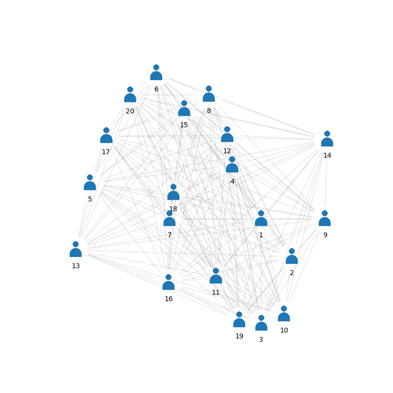
Items: \(\{1, 2, \ldots, n\}\)
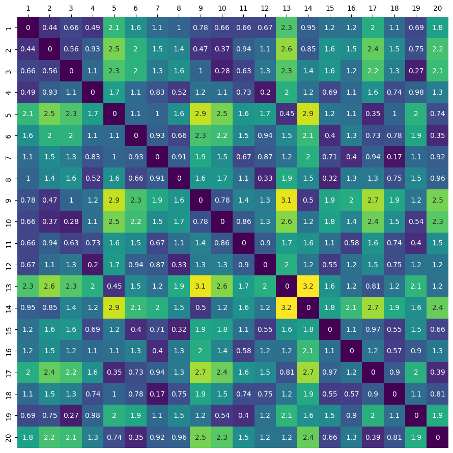
\[ \Delta= (\delta_{ij})_{1 \leq i,j \leq n} \in \mathbb{R}^{n \times n} \]

Multidimensional Scaling (MDS)

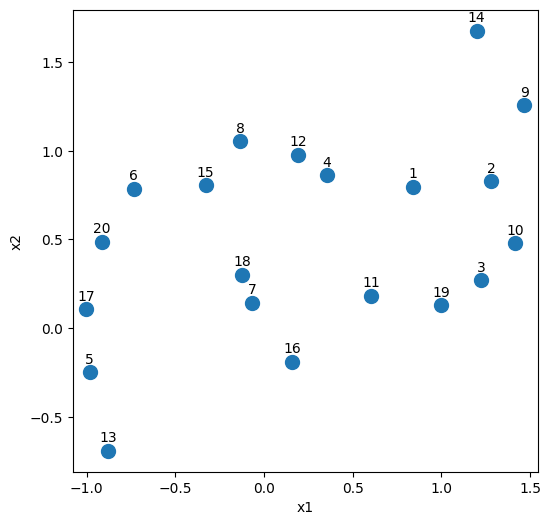
  • Given pairwise dissimilarity data \(\Delta= (\delta_{ij}) \in \mathbb{R}^{n \times n}\) and an embedding dimension* \(p \ll n\)
  • Find a configuration of points \(\{ \widehat{x}_1, \dots, \widehat{x}_n\} \in \mathbb{R}^p\) such that:

\(\displaystyle\| \widehat{x}_i - \widehat{x}_j \|^2 \approx \delta_{ij} \quad \text{ for all } 1 \leq i,j \leq n\)

*usually \(p=2\) or \(p=3\)

\(\longrightarrow\)

\(\longrightarrow\)
Multidimensional Scaling (MDS)
Classical MDS (CMDS) Algorithm

Given: dissimilarity matrix \(\Delta= (\delta_{ij}) \in \mathbb{R}^{n \times n}\) and \(p \ll n\)

  1. Double centering:

\(\Delta_c= -\frac{1}{2}H \Delta H\quad\) where \(\quad H = \Big(I_n - \frac{1}{n}\boldsymbol{1}_n \boldsymbol{1}_n^{\mathsf{T}}\Big)\)

  1. Rank-p spectral decomposition:

\(\Delta_c= {\widehat{U}}\widehat{\Lambda }{\widehat{U}}^{\mathsf{T}}+ \widehat{V}_{\perp} \widehat{\Lambda}_{\perp} \widehat{V}_{\perp}^{\mathsf{T}}\)

  1. Spectral embedding:

\(\widehat{X}= {\widehat{U}}\widehat{\Lambda}^{1/2}\)

Output: embedding \(\widehat{X}\in \mathbb{R}^{n \times p}\)

\(\Delta\in \mathbb{R}^{n \times n}\)
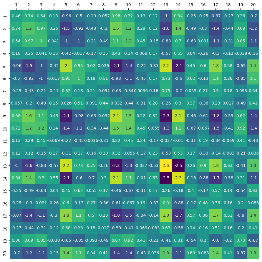
\(\Delta_c\in \mathbb{R}^{n \times n}\)
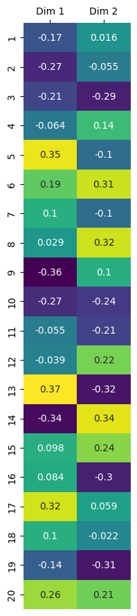
\({\widehat{U}}\in \mathbb{R}^{n \times p}\)
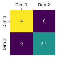
\(\widehat{\Lambda}\in \mathbb{R}^{p \times p}\)
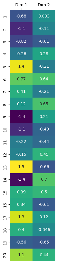
\(\widehat{X}\in \mathbb{R}^{n \times p}\)

Dates back to (Young and Householder 1938). Later rediscovered by (Torgerson 1952) and (Gower 1966).

Identifiability of MDS Embeddings

  • In the realizable setting, there exists a latent configuration \(\color{green}{x_1, \dots, x_n} \in \mathbb{R}^p\) such that \(\color{green}{\delta_{ij} = \|x_i - x_j\|^2}\)

  • Let \(\color{green}{X} \in \mathbb{R}^{n \times p}\) be the configuration matrix

  • For any rigid transformation \(g \in \mathcal{G}\) (i.e., rotation + reflection + translation),    \(\color{green}{\Delta\big(\color{green}{X}\big)} \equiv \color{green}{\Delta\big(}\color{magenta}{g}(\color{green}{X)\big)}\)

Theorem (Young and Householder 1938; Schoenberg 1935).

In the realizable setting, the CMDS algorithm exactly recovers the latent configuration up to rigid transformations, i.e.,

\[ \mathsf{CMDS}\big(\; \color{green}{\color{green}{\Delta(X)}}, p\;\big) = \color{magenta}{g}(\color{green}{X}) \quad \text{ for some } \color{magenta}{g} \in \mathcal{G} \]

(a short proof is in the appendix)

MDS under noise

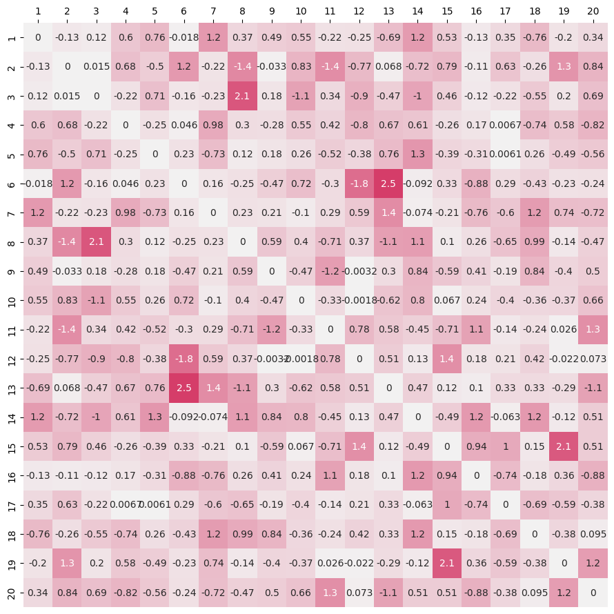
In practice, the dissimilarity data is often subject to noise and/or measurement errors, i.e., we observe: \[ \begin{aligned} d_{ij} &= \color{green}{\delta_{ij}} + \color{red}{\varepsilon_{ij}}\\ D &= \underbrace{\color{green}{\Delta}}_{\color{green}{\text{signal}}} + \underbrace{\color{red}{\mathcal{E}}}_{\color{red} {\text{noise}}} \end{aligned} \]
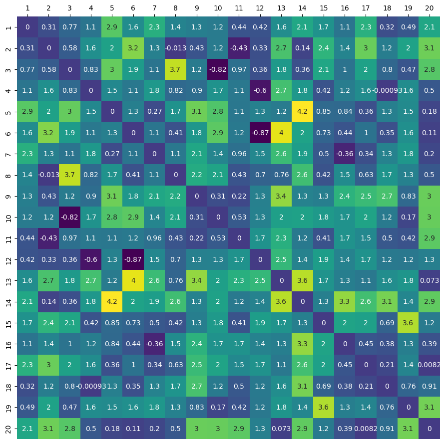
\(=\)
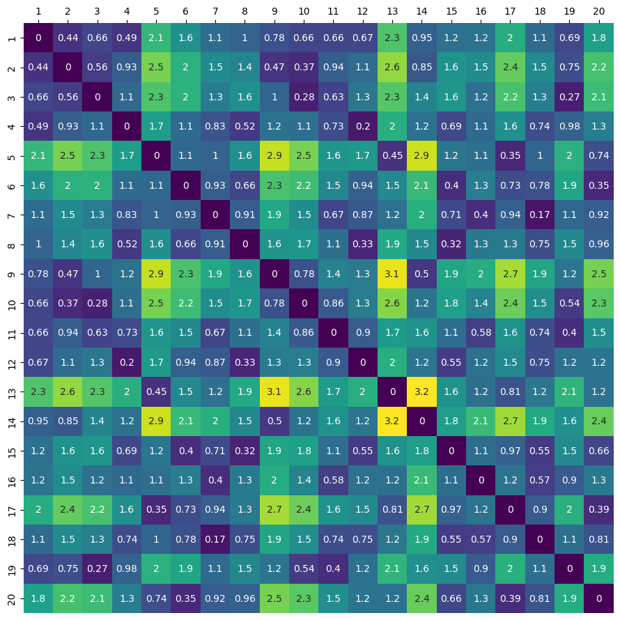
\(+\)
MDS under noise

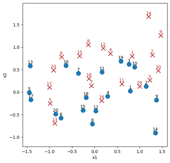
In practice, the dissimilarity data is often subject to noise and/or measurement errors, i.e., we observe: \[ \begin{aligned} d_{ij} &= \color{green}{\delta_{ij}} + \color{red}{\varepsilon_{ij}}\\ D &= \underbrace{\color{green}{\Delta}}_{\color{green}{\text{signal}}} + \underbrace{\color{red}{\mathcal{E}}}_{\color{red} {\text{noise}}} \end{aligned} \]


  • \(\color{green}{X}\) is the configuration matrix underlying the signal \(\Delta\)
  • \(\widehat{X}= \mathsf{CMDS}(D, p)\) is the CMDS embedding of \(D\)

The noisy CMDS embedding \(\widehat{X}\) reflects the variability in \(D\) due to \(\color{red}{\mathcal{E}}\)
Desiderata - I (Statistical Learning)

  • Let \(D = \color{green}{\Delta(X)}+ \color{red}{\mathcal{E}}\) and \(\widehat{X}= \mathsf{CMDS}(D, p)\)
  • For any metric \(\|\widehat{X}- \color{green}{X}\|_{\dagger}\), define the reconstruction error*:

\(\displaystyle\ell(\widehat{X}, \color{green}{X}) = \min_{g \in \mathcal{G}} \| g(\widehat{X}) -\color{green}{X}\|_{\dagger}\)

1. Can we recover the signal with high probability? i.e.,

\[ \mathbb{P}\Big(\; \ell(\widehat{X},\color{green}{X}) \lesssim R_n \;\Big) \geq 1 - \alpha_n \quad \text{ for } R_n, \alpha_n \to 0 \]

2. How do the configuration \(\color{green}{X}\) and the noise \(\color{red}{\mathcal{E}}\) impact \(\ell(\widehat{X},\color{green}{X})\)?

3. Can we do better than the CMDS algorithm?


*modulo rigid transformations

Example - 1: Sensor Localization

Suppose \(n\) sensors are placed in various locations across the United States, and \[ d_{ij} = \color{red}{\text{noisy}} \text{ squared Euclidean distance between sensors $i$ and $j$} \]
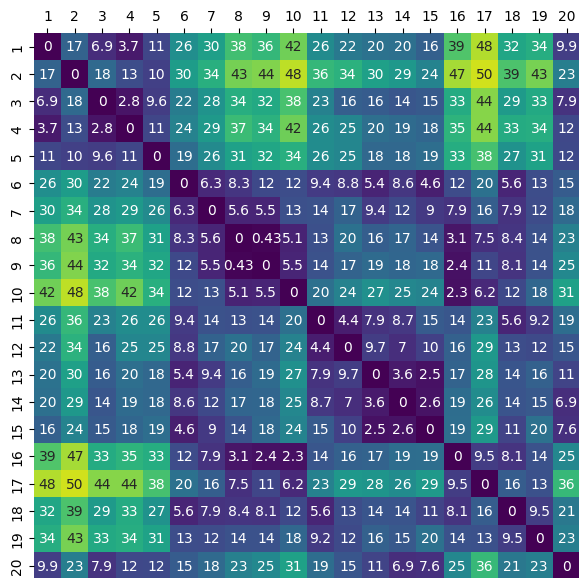
Are the sensors placed in the following locations?

  • San Diego, CA
  • Phoenix, AZ
  • \(\dots\)
  • Washington, DC

\[ \mathbb{P}\Big( \text{locations}(d_{ij}) \simeq \{\text{San Diego}, \dots, \text{Washington DC}\} \Big)? \]

Example - 1

This tells us:

\(\quad\quad\) \(\ell(\displaystyle\widehat{X},\; \color{green}{X}) \lesssim R_n\) with probability at least \(1-\alpha_n\)

Example - 1

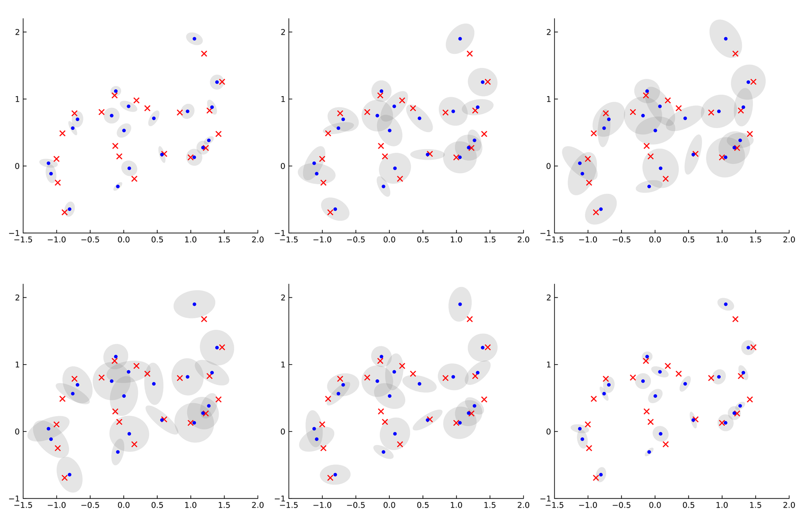
It would be nice to have some set \(\color{Purple}{\mathcal{C}_\alpha}\) such that:

\(\mathbb{P}(\displaystyle\color{green}{X}\in {\color{Purple}{\mathcal{C}_{\alpha}}}) \approx 1-\alpha\)

Desiderata - II (Uncertainty Quantification)

  • For any \(\color{DarkOrange}{\boldsymbol{\alpha}} \in (0, 1)\)
  • Can we construct \(\color{DarkOrange}{\boldsymbol{100 \times (1-\alpha)\%}}\) uniform confidence sets \[ \mathcal{C}_{\alpha} = \prod_{i=1}^n \mathcal{C}_{\alpha, i} \subset \mathbb{R}^p \] which provide simultaneous coverage* of the true configuration: \[ \boxed{\phantom{\Bigg()} \mathbb{P}\Big( \exists g \in \mathcal{G}: \; g(\color{green}{x_i}) \in \mathcal{C}_{\alpha, i} \;\;\; \color{Purple}{\forall i \in [n]} \Big) \approx \color{DarkOrange}{\boldsymbol{1 - \alpha}} \phantom{\Bigg()}} \]
*modulo rigid transformations

Statistical Learning

\(\displaystyle D = \color{green}{\Delta(X)}+ \color{red}{\mathcal{E}}\quad \text{for} \quad \color{green}{X}\in \mathbb{X}({\kappa, \varpi})\)

Assumptions on \(\color{green}{X}\)
Compactly supported \(\|{\color{green}{X}}\|_{2\to\infty} \le \varpi\)
Bounded condition number \(\hspace{0em}\) \(\kappa^{-1}\le s_p\left(\tfrac{\color{green}{X}}{\sqrt{n}}\right) \le s_1\left(\tfrac{\color{green}{X}}{\sqrt{n}}\right) \le \kappa\)
Assumptions on \(\color{red}{\mathcal{E}}\)
Independent \(\hspace{1.4em}\) \((\color{red}{\varepsilon_{ij}})\) are independent for \(i < j\) \(\hspace{1.4em}\)
Heteroscedastic \(\mathbb{E}(\color{red}{\varepsilon_{ij}}) = 0\) and \(\text{Var}(\color{red}{\varepsilon_{ij}}) = \sigma_{ij}^2\)
Finite \(q^{\text{th}}\) moment For \(q > 4,\quad\) \(\displaystyle\max_{i < j}\|\color{red}{\varepsilon_{ij}}\|_{L^q} \le \sigma\)

Examples \(\hspace{3em}\)

\[ \begin{aligned} d_{ij} &= \color{green}{\delta_{ij}} + \color{red}{\xi_{ij}} &&\hspace{3em} (\text{additive})\\ d_{ij} &= \color{green}{\delta_{ij}} + \color{red}{\delta_{ij}\xi_{ij}} &&\hspace{3em} (\text{multiplicative})\\ \log d_{ij} &= \log \color{green}{\delta_{ij}} + \color{red}{\xi_{ij}} &&\hspace{3em} (\text{log-Normal})\\ d_{ij} &= \color{green}{\delta_{ij}} + \color{red}{2\delta_{ij}\xi_{ij} + \xi_{ij}^2} &&\hspace{3em} (\text{absolute additive})\\ \end{aligned} \] where \({\Xi = (\xi_{ij})}\) is a random matrix with iid entries

Signal Recovery

\(\color{green}{X}\in \mathbb{X}({\kappa, \varpi}) \hspace{2em} D = \color{green}{\Delta(X)}+ \color{red}{\mathcal{E}}; \hspace{2em} \widehat{X}= \mathsf{CMDS}(D, p); \hspace{2em} \text{and} \quad \color{brown}{\overset{\mathbf{\smallsmile}}{X}}(D) \in \mathbb{R}^{n \times p}\) be any estimator of \(\color{green}{X}\)

(Lower Bound). The reconstruction error \(\ell(\widehat{X},\color{green}{X})\) has:

  • lower bound \(r_n \to 0\), if:

\[ \sup_{D = \color{green}{\Delta(X)}+ \color{red}{\mathcal{E}}}\mathbb{P}\Big(\;\; \ell(\color{brown}{\overset{\mathbf{\smallsmile}}{X}},\,\color{green}{X}) \gtrsim r_n \;\;\Big) \ge \frac{1}{2} \]

(Minimax Lower Bound). The reconstruction error \(\ell(\widehat{X},\color{green}{X})\) has:

  • minimax lower bound \(r_n \to 0\), if:

\[ \inf_{\color{brown}{\overset{\mathbf{\smallsmile}}{X}}} \sup_{D = \color{green}{\Delta} + \color{red}{\mathcal{E}}} \mathbb{P}\Big(\;\; \ell(\color{brown}{\overset{\mathbf{\smallsmile}}{X}},\,\color{green}{X}) \gtrsim r_n\;\; \Big) \ge \frac{1}{2} \]

(CMDS Upper Bound). The reconstruction error \(\ell(\widehat{X},\color{green}{X})\) has:

  • convergence rate \(R_n \to 0\)
  • with failure probability \(\alpha_n \to 0\), if:

\[ \sup_{D = \color{green}{\Delta(X)}+ \color{red}{\mathcal{E}}}\mathbb{P}\Big(\;\; \ell(\widehat{X},\color{green}{X}) \gtrsim R_n \;\;\Big) \leq \alpha_n \]

Reconstruction metrics
RMSE

\(\displaystyle\ell_\text{RMSE}(\widehat{X},\color{green}{X}) = \frac{1}{\sqrt{n}}\|g(\widehat{X}) - X\|_F\)
\(2\)-to-\(\infty\) uniform error

\(\displaystyle\ell_{2\to\infty}(\widehat{X},\color{green}{X}) = \max_{i \in [n]} \|g(\widehat{x}_i) - x_i\|\)

Minimax Lower Bound      CMDS Upper Bound
\(\displaystyle \inf_{\color{brown}{\overset{\mathbf{\smallsmile}}{X}}} \sup_{D = \color{green}{\Delta(X)}+ \color{red}{\mathcal{E}}} \mathbb{P}\Big(\;\; \ell(\color{brown}{\overset{\mathbf{\smallsmile}}{X}},\,\color{green}{X}) \gtrsim r_n\;\; \Big) \ge \frac{1}{2}\) \(\displaystyle \sup_{D = \color{green}{\Delta(X)}+ \color{red}{\mathcal{E}}}\mathbb{P}\Big(\;\; \ell(\widehat{X}, \color{green}{X}) \gtrsim R_n \;\;\Big) \;\le\; \alpha_n\)

Theorem (Vishwanath and Arias-Castro 2025b).   For all   \(0 < r < \frac{q-4}{2}\):

Metric Lower bound \(r_n\)    Upper bound \(R_n\)    Failure Probability \(\alpha_n\)
\[\ell_\text{RMSE}\] \(\displaystyle\frac{\sigma\kappa}{\sqrt{n}}\) \(\displaystyle\frac{\sigma\kappa}{\sqrt{n}}\)
\(O(n^{-2} + n^{-r})\)
\(\ell_{_{2\to\infty}}\) \(\displaystyle\underline{c}({\kappa, \varpi})\cdot \sigma\sqrt{\frac{\log{n}}{n}}\) \(\displaystyle\overline{c}({\kappa, \varpi})\cdot \sigma\sqrt{\frac{\log{n}}{n}}\) \(O(n^{-2} + n^{-r})\)

  • \(q > 4\) moments is necessary for consistency
  • Parametric rates (in \(n\)) for \(\ell_\text{RMSE}\) and minimax-optimal up to absolute constants. Extra \(\sqrt{\log{n}}\) factor for \(\ell_{_{2\to\infty}}\) is unavoidable
  • Proof relies on: (1.) orthogonal Procrustes alignment + (2.) Fuk-Nagaev-type matrix concentration

where   \(\overline{c}({\kappa, \varpi}) = \kappa^2(\kappa + \varpi)\)   and   \(\underline{c}({\kappa, \varpi}) = \kappa(1+\kappa\varpi)^{-1}\).

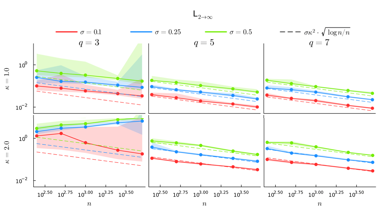
Illustration

Uncertainty Quantification

Desiderata - II (Uncertainty Quantification)

  • For any \(\color{DarkOrange}{\boldsymbol{\alpha}} \in (0, 1)\)
  • Can we construct \(\color{DarkOrange}{\boldsymbol{100 \times (1-\alpha)\%}}\) uniform confidence sets \[ \mathcal{C}_{\alpha} = \prod_{i=1}^n \mathcal{C}_{\alpha, i} \subset \mathbb{R}^p \] which provide simultaneous coverage* of the true configuration: \[ \boxed{\phantom{\Bigg()} \mathbb{P}\Big( \exists g \in \mathcal{G}: \; g(\color{green}{x_i}) \in \mathcal{C}_{\alpha, i} \;\;\; \color{Purple}{\forall i \in [n]} \Big) \approx \color{DarkOrange}{\boldsymbol{1 - \alpha}} \phantom{\Bigg()}} \]

*modulo rigid transformations

Tail bounds don’t suffice

Let \(\color{green}{X}\in \mathbb{X}({\kappa, \varpi})\) and \(D = \color{green}{\Delta}+ \color{red}{\mathcal{E}}\), and let \(\widehat{X}= \mathsf{CMDS}(D, p)\)

Tail bound. The constant \(\color{red}{C_1}\) is unknown and is going to be too conservative for practical use

\[ \begin{aligned} &\mathbb{P}\bigg( \|{\widehat{X}- \widehat{g}(X)}\|_{2\to\infty} \ge \color{red}{C_1} \;\cdot\; \underline{c}({\kappa, \varpi}) \sigma\;\cdot \sqrt{\tfrac{t + \log{n}}{n}} \bigg) \le e^{-t}\\ \phantom{\implies} &\phantom{\mathbb{P}\bigg( \|{\widehat{X}- \color{magenta}{\widehat{g}}(X)}\|_{2\to\infty} \le \color{red}{C_1} \;\cdot\; \underline{c}({\kappa, \varpi}) \sigma\;\cdot \sqrt{\tfrac{\log(1/\alpha) + \log{n}}{n}} \bigg) \ge 1-\alpha} \end{aligned} \]

Tail bound. The constant \(\color{red}{C_1}\) is unknown and is going to be too conservative for practical use

\[ \begin{aligned} &\mathbb{P}\bigg( \|{\widehat{X}- \color{magenta}{\widehat{g}}(X)}\|_{2\to\infty} \ge \color{red}{C_1} \;\cdot\; \underline{c}({\kappa, \varpi}) \sigma\;\cdot \sqrt{\tfrac{t + \log{n}}{n}} \bigg) \le e^{-t}\\ \implies &\mathbb{P}\bigg( \|{\widehat{X}- \color{magenta}{\widehat{g}}(X)}\|_{2\to\infty} \le \color{red}{C_1} \;\cdot\; \underline{c}({\kappa, \varpi}) \sigma\;\cdot \sqrt{\tfrac{\log(1/\alpha) + \log{n}}{n}} \bigg) \ge 1-\alpha \end{aligned} \]

Distributional approximation. Let \(\widehat{{F}}\) be an estimate for the distribution of \(\|{\widehat{X}- \color{magenta}{\widehat{g}}(X)}\|_{2\to\infty}\). The constant \(\color{red}{C_2}\) does not impact its practical use

\[ \begin{aligned} &\sup_{t \in \mathbb{R}}\bigg|\;\;{\mathbb{P}\big( \|{\widehat{X}- \color{magenta}{\widehat{g}}(X)}\|_{2\to\infty} \le t \big) - \mathbb{P}(\widehat{{F}} \le t)}\;\;\bigg| \le \color{red}{C_2} \mathfrak{R}_n\\ \phantom{\implies} &\phantom{\mathbb{P}\bigg( \|{\widehat{X}- \color{magenta}{\widehat{g}}(X)}\|_{2\to\infty} \le q_{1-\alpha}(\widehat{{F}}) \bigg) \ge 1-\alpha - \color{red}{C_2} \mathfrak{R}_n} \end{aligned} \]

where \(\mathfrak{R}_n \to 0\)

Distributional approximation. Let \(\widehat{{F}}\) be an estimate for the distribution of \(\|{\widehat{X}- \color{magenta}{\widehat{g}}(X)}\|_{2\to\infty}\). The constant \(\color{red}{C_2}\) does not impact its practical use

\[ \begin{aligned} &\sup_{t \in \mathbb{R}}\bigg|\;\;{\mathbb{P}\big( \|{\widehat{X}- \color{magenta}{\widehat{g}}(X)}\|_{2\to\infty} \le t \big) - \mathbb{P}(\widehat{{F}} \le t)}\;\;\bigg| \le \color{red}{C_2} \mathfrak{R}_n\\ \implies &\mathbb{P}\bigg( \|{\widehat{X}- \color{magenta}{\widehat{g}}(X)}\|_{2\to\infty} \le q_{1-\alpha}(\widehat{{F}}) \bigg) = 1-\alpha \pm \color{red}{C_2} \mathfrak{R}_n \end{aligned} \]

where \(\mathfrak{R}_n \to 0\) and by setting \(t = q_{1-\alpha}(\widehat{{F}})\)

Extreme value distributional approximation

Theorem (Vishwanath and Arias-Castro 2025a). Let \(\widehat{\Omega}_i\) be the covariance matrix around each \(\widehat{x}_i\), and the normalized \(\ell_{2\to\infty}\)-error: \[ T_n := \sqrt{n}\; \cdot\; \max_{i \in [n]} \|\;\;\widehat{\Omega}_i^{-1/2}\left(x_i - \color{magenta}{\widehat{g}}(\widehat{x}_i)\right)\;\;\| \]

1. Convergence. Let \(G\) denote a Gumbel random variable. Then, there exist deterministic sequences* \((a_n)\) and \((b_n)\) such that

\[ \sup_{t \in \mathbb{R}}\Bigg|\;\; \mathbb{P}\Big( \tfrac{T_n - b_n}{a_n} \le t \Big) - \mathbb{P}\big( G \le t \big) \;\; \Bigg| \lesssim \frac{\log\log{n}}{\log{n}} \]

2. Confidence set. For a confidence level \(1-\alpha\), let \(q_{1-\alpha}\) be the \((1-\alpha)\) Gumbel quantile, and consider the ellipsoids

\[ \mathcal{C}_{\alpha, i} := \mathscr{E}\Big( \underbrace{\widehat{x}_i}_{\text{center}},\; \underbrace{\widehat{\Omega}_i}_{\text{shape}},\;\; \underbrace{b_n + a_n q_{1-\alpha}}_{\text{generalized radius}} \Big) \]

\(\displaystyle\mathbb{P}\Big( \color{magenta}{\widehat{g}}(x_i) \in \mathcal{C}_{\alpha, i} \; \forall i \in [n] \Big) = 1 - \alpha \pm O\Big(\frac{\log\log{n}}{\log{n}}\Big)\)

Details about \(\widehat{\Omega}_i\) in the appendix.      Compare    \(T_n\)    with    \(\displaystyle\sqrt{n} \cdot \ell_{2\to\infty}= \sqrt{n} \;\cdot\; \max_{i \in [n]} \|\;\; \left(x_i - \color{magenta}{\widehat{g}}(\widehat{x}_i) \right) \;\;\|\)

\(\quad\) \(b_n^2 = {2\log{n} + (p-2)\log\log{n} - 2\log{\Gamma(p/2)}}\)     and     \(a_n = 1/b_n\)    

Extreme value distributional approximation

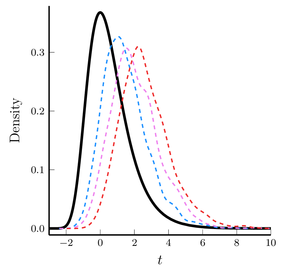
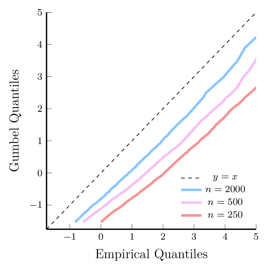
\(\frac{T_n - b_n}{a_n}\quad\) vs. \(\quad G\)
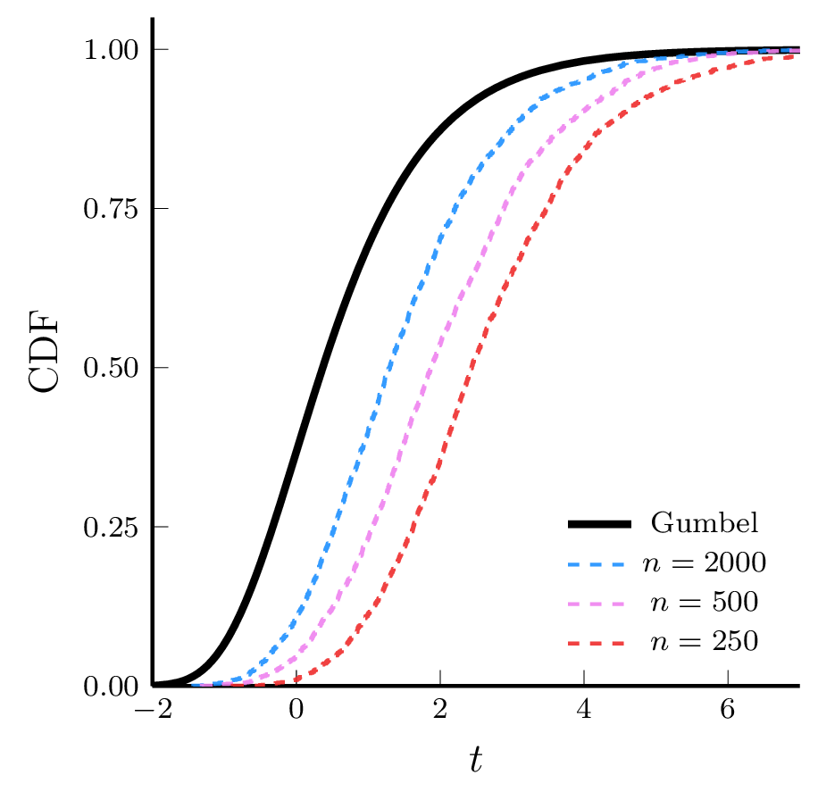
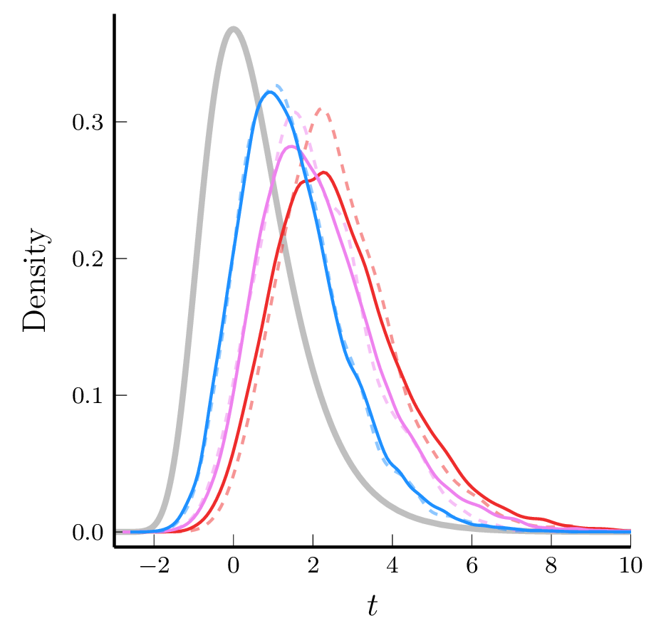
\(O\left(\tfrac{\log\log{n}}{\log{n}}\right)\) convergence rate is extremely slow!

Bootstrap confidence sets

Given: \(D = \color{green}{\Delta}+ \color{red}{\mathcal{E}}\)

1. \(\widehat{X}= \mathsf{CMDS}(D, p)\)

2. Compute the residuals \(\color{purple}{E} = D - \Delta(\widehat{X})\)

3. For \(b = 1, \ldots, B\):

  3.1 Externally randomize \(\color{purple}{E}\) to get \(\color{red}{\mathcal{E}}^{\flat}\)

      • Empirical bootstrap:   \(\color{red}{\varepsilon_{ij}} \sim_{\text{iid}} (e_{ij})\) with replacement

      • Multiplier bootstrap: \(\color{red}{\varepsilon_{ij}} = e_{ij} \cdot r_{ij}\) where \(r_{ij} \sim_{\text{iid}} N(0, 1)\)

  3.2 Generate noisy dissimilarities \(D^{\flat}= \Delta(\widehat{X}) + \color{red}{\mathcal{E}}^{\flat}\)

  3.3 Compute \(\widehat{X}^{\flat}= \mathsf{CMDS}(D^{\flat}, p)\)

  3.4 Compute \(\widehat T_n^{\flat}= \max_{i}\|\widehat{\Omega}^{-1/2}(\widehat{x}_i - \color{magenta}{\widehat{g}}^{\flat}(\widehat{x}_i^{\flat}))\|\) via Procrustes

4. Compute the bootstrap quantile  \(q_{1-\alpha}^{\flat}\)  of   \(\{\widehat T_n^{\flat}(1), \dots, \widehat T_n^{\flat}(B)\}\)

Return: \(\displaystyle\mathcal{C}_{\alpha, i} := \mathscr{E}\big( \widehat{x}_i,\; \widehat{\Omega}_i,\;\; q^{\flat}_{1-\alpha} \big)\) for \(i=1, \dots, n\)

\(D \in \mathbb{R}^{n \times n}\)
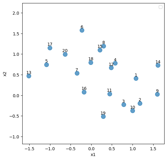

\(\widehat{X}\in \mathbb{R}^{n \times p}\)

\(E \in \mathbb{R}^{n \times n}\)
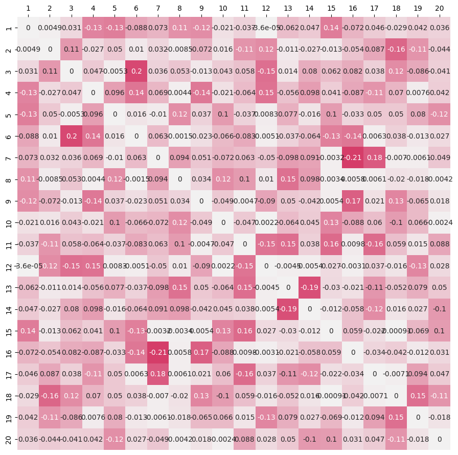
\(\mathcal{E}^{\flat}\in \mathbb{R}^{n \times n}\)

\(D^{\flat}\in \mathbb{R}^{n \times n}\)
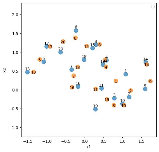

\(\widehat{X}^{\flat}\in \mathbb{R}^{n \times p}\)

Bootstrap distributional approximation

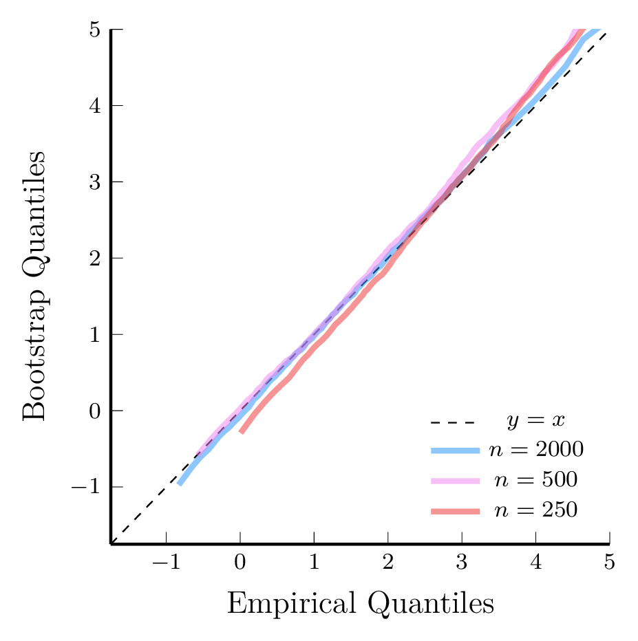
\({T_n}\quad\) vs. \(\quad T_n^{\flat}\)
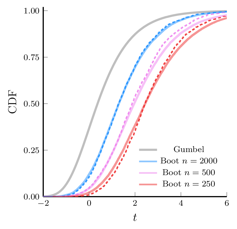
The bootstrap distributional approximation is substantially better!

Bootstrap distributional approximation

Theorem (Vishwanath and Arias-Castro 2025a). Let \(T_n\) and \(T_n^{\flat}\) be given by:

     \(\displaystyle T_n = \sqrt{n}\;\cdot\;\max_{i \in [n]}\|\;\;\widehat{\Omega}_i^{-1/2}\big(x_i - \color{magenta}{\widehat{g}}(\widehat{x}_i)\big)\;\;\|\)    and    \(\displaystyle T_n^{\flat}= \sqrt{n}\;\cdot\;\max_{i \in [n]} \|\;\;\widehat{\Omega}_i^{-1/2}\big(\widehat{x}_i - \color{magenta}{\widehat{g}}^{\flat}(\widehat{x}_i^{\flat})\big)\;\;\|\)


1. Convergence. With probability \(1-O(n^{-2})\) over the randomness in \(\mathcal{E}\),

\[ \sup_{t \in \mathbb{R}}\Bigg|\;\; \mathbb{P}\big(T_n \le t \big) - \mathbb{P}\big(T_n^{\flat}\le t \big) \;\;\Bigg| \lesssim \color{brown}{\frac{\log^5{n}}{{\sqrt{n}}}} \]


2. Confidence set. For a confidence level \(1-\alpha\), let \(q^{\flat}_{1-\alpha}\) be the \((1-\alpha)\) Bootstrap quantile, and consider the ellipsoids

\[ \mathcal{C}^{\flat}_{\alpha, i} := \mathscr{E}\Big( \widehat{x}_i,\; \widehat{\Omega}_i,\;\; q^{\flat}_{1-\alpha} \Big) \]

\(\displaystyle\mathbb{P}\Big( \color{magenta}{\widehat{g}}(x_i) \in \mathcal{C}^{\flat}_{\alpha, i} \; \forall i \in [n] \Big) = 1 - \alpha \pm O\Big(\color{brown}{\frac{\log^5{n}}{{\sqrt{n}}}}\Big)\)

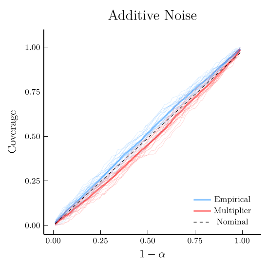
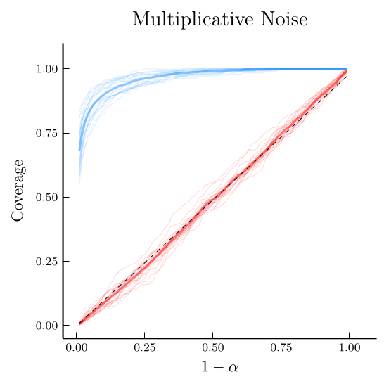
Bootstrap Example

\(X\in \mathbb{X}\) is chosen inside an ellipsoid with \(\kappa=2\) and \(d_{ij} = \color{green}{\delta_{ij}} + \color{red}{\varepsilon_{ij}}\) multiplicative/additive noise

\(\color{red}{\varepsilon_{ij}} \sim N(0, 1)\)
\(\color{red}{\varepsilon_{ij}} \sim N(0, \delta_{ij}^2)\)
Example - 2: Senate Voting

Senators’ voting records in the 116th U.S. Congress from 2019–2021 (Lewis et al. 2019) \[ d_{ij} = \% \text{disagreement between senators $i$ and $j$ on roll-call votes} \] \(D = (d_{ij}) \in \mathbb{R}^{100 \times 100}\) and let \(\widehat{X}= \mathsf{CMDS}(D, 2) \in \mathbb{R}^{100 \times 2}\) be the embedding

Example - 2

Senators’ voting records in the 116th U.S. Congress from 2019–2021 (Lewis et al. 2019) \[ d_{ij} = \% \text{disagreement between senators $i$ and $j$ on roll-call votes}. \] \(D = (d_{ij}) \in \mathbb{R}^{100 \times 100}\) and let \(\widehat{X}= \mathsf{CMDS}(D, 2) \in \mathbb{R}^{100 \times 2}\) be the embedding

Intuition behind extreme value approximation

\(\boxed{ T_n := \sqrt{n}\; \cdot\; \max_{i \in [n]} \|\;\;\color{red}{\widehat{\Omega}_i^{-1/2}\left(x_i - \widehat{g}(\widehat{x}_i)\right)}\;\;\| }\)

For each fixed \(i \in [n]\): \[ \begin{aligned} \sqrt{n} \cdot \color{red}{\widehat{\Omega}_i^{-1/2}\left(x_i - \widehat{g}(\widehat{x}_i)\right)} &= \frac{1}{\sqrt{n}} \sum_{j=1}^n \varepsilon_{ij}x_j \;\; + \underbrace{h_n}_{\text{higher order terms}}\\ \phantom{\sqrt{n} \cdot \color{red}{\widehat{\Omega}_i^{-1/2}\left(x_i - \widehat{g}(\widehat{x}_i)\right)}} &\phantom{\;\approx\; \frac{1}{\sqrt{n}} (\varepsilon_{i1}x_1 + \varepsilon_{i2} x_2 + \dots + \varepsilon_{in}x_n) \;\longrightarrow\; N(0, I_p)} \end{aligned} \]

For each fixed \(i \in [n]\) \[ \begin{aligned} \sqrt{n} \cdot \color{red}{\widehat{\Omega}_i^{-1/2}\left(x_i - \widehat{g}(\widehat{x}_i)\right)} &\;\approx\; \frac{1}{\sqrt{n}} (\varepsilon_{i1}x_1 + \varepsilon_{i2} x_2 + \dots + \varepsilon_{in}x_n) \;\longrightarrow\; N(0, I_p)\\ \phantom{\sqrt{n}\cdot \|\color{red}{\widehat{\Omega}_i^{-1/2}\left(x_i - \widehat{g}(\widehat{x}_i)\right)}\| } &\phantom{\;\approx\; \frac{1}{\sqrt{n}} \|\varepsilon_{i1}x_1 + \varepsilon_{i2} x_2 + \dots + \varepsilon_{in}x_n\| \;\longrightarrow\; \chi_p} \end{aligned} \]

For each fixed \(i \in [n]\) \[ \begin{aligned} \sqrt{n} \cdot \color{red}{\widehat{\Omega}_i^{-1/2}\left(x_i - \widehat{g}(\widehat{x}_i)\right)} &\;\approx\; \frac{1}{\sqrt{n}} (\varepsilon_{i1}x_1 + \varepsilon_{i2} x_2 + \dots + \varepsilon_{in}x_n) \;\longrightarrow\; N(0, I_p)\\ \sqrt{n}\cdot \|\;\color{red}{\widehat{\Omega}_i^{-1/2}\left(x_i - \widehat{g}(\widehat{x}_i)\right)}\;\| &\;\approx\; \frac{1}{\sqrt{n}} \|\varepsilon_{i1}x_1 + \varepsilon_{i2} x_2 + \dots + \varepsilon_{in}x_n\| \;\longrightarrow\; \chi_p \end{aligned} \]

\[ \begin{aligned} \sqrt{n}\cdot \|\;\color{red}{\widehat{\Omega}_1^{-1/2}\left(x_1 - \widehat{g}(\widehat{x}_1)\right)}\;\| &\;\approx\; \frac{1}{\sqrt{n}} \|\varepsilon_{11}x_1 + \varepsilon_{12} x_2 + \dots + \varepsilon_{1n}x_n\| \;\longrightarrow\; \chi_p\\ \sqrt{n}\cdot \|\;\color{red}{\widehat{\Omega}_2^{-1/2}\left(x_2 - \widehat{g}(\widehat{x}_2)\right)}\;\| &\;\approx\; \frac{1}{\sqrt{n}} \|\varepsilon_{21}x_1 + \varepsilon_{22} x_2 + \dots + \varepsilon_{2n}x_n\| \;\longrightarrow\; \chi_p\\[0.5em] \vdots\quad\quad &\;\approx\; \quad\quad\vdots\\[0.5em] \sqrt{n}\cdot \|\;\color{red}{\widehat{\Omega}_n^{-1/2}\left(x_n - \widehat{g}(\widehat{x}_n)\right)}\;\| &\;\approx\; \frac{1}{\sqrt{n}} \|\varepsilon_{n1}x_1 + \varepsilon_{n2} x_2 + \dots + \varepsilon_{nn}x_n\| \;\longrightarrow\; \chi_p \end{aligned} \]

Maximum of independent \(\chi_p\) random variables converges to Gumbel at rate \(O\left(\frac{1}{\log{n}}\right)\)

\[ \begin{aligned} \sqrt{n}\cdot \|\;{\widehat{\Omega}_1^{-1/2}\left(x_1 - \widehat{g}(\widehat{x}_1)\right)}\;\| &\;\approx\; \frac{1}{\sqrt{n}} \|0x_1 + \color{lime}{\varepsilon_{12}} x_2 + \dots + \color{brown}{\varepsilon_{1n}}x_n\| \;\longrightarrow\; \chi_p\\ \sqrt{n}\cdot \|\;{\widehat{\Omega}_2^{-1/2}\left(x_2 - \widehat{g}(\widehat{x}_2)\right)}\;\| &\;\approx\; \frac{1}{\sqrt{n}} \|\color{lime}{\varepsilon_{21}}x_1 + 0 x_2 + \dots + \color{magenta}{\varepsilon_{2n}}x_n\| \;\longrightarrow\; \chi_p\\[0.5em] \vdots\quad\quad &\;\approx\; \quad\quad\vdots\\[0.5em] \sqrt{n}\cdot \|\;{\widehat{\Omega}_n^{-1/2}\left(x_n - \widehat{g}(\widehat{x}_n)\right)}\;\| &\;\approx\; \frac{1}{\sqrt{n}} \|\color{brown}{\varepsilon_{n1}}x_1 + \color{magenta}{\varepsilon_{n2}} x_2 + \dots + 0x_n\| \;\longrightarrow\; \chi_p \end{aligned} \]

The random variables in \(T_n\) are not independent! The main proof uses:
(i) Chen-Stein Poisson approximation   (ii) a local anti-concentration inequality for Gaussian quadratic forms

Why the bootstrap approximation is better

Population world

We observe \(D = \color{green}{\color{green}{\Delta(X)}} + \color{red}{\mathcal{E}}\phantom{{}^{\flat}}\) and \(\widehat{X}= \mathsf{CMDS}(D, p)\phantom{\widehat T_n^{\flat}}\)

Bootstrap world

We observe \(D^{\flat}= \color{green}{\Delta(\widehat{X})} + \color{red}{\mathcal{E}}^{\flat}\) and \(\widehat{X}^{\flat}= \mathsf{CMDS}(D^{\flat}, p)\)


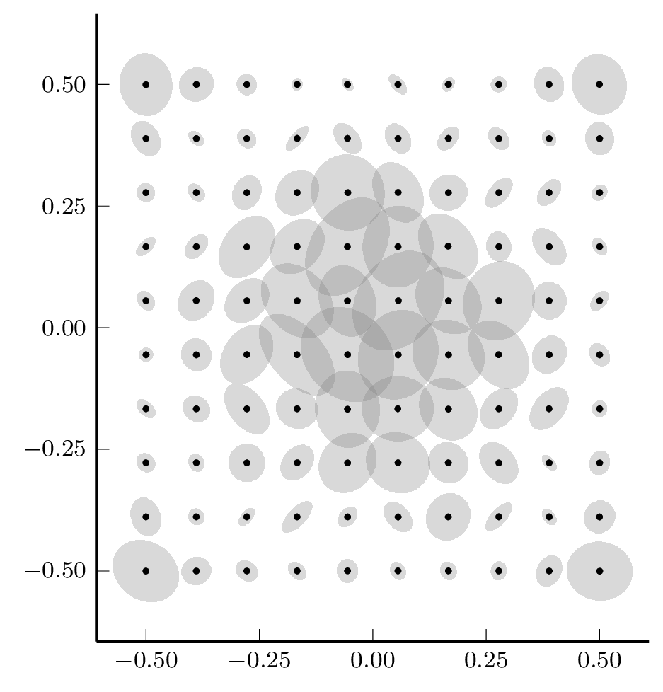
Adaptivity of Multiplier Bootstrap to Heteroscedasticity

\(X\in \mathbb{X}\) is uniformly spaced on a grid and \(d_{ij} = \color{green}{\delta_{ij}} + \color{red}{\varepsilon_{ij}}\) with radial sum/difference noise:

\(\color{red}{\varepsilon_{ij}} \sim N(0, \|x_i\|^2 + \|x_j\|^2)\)
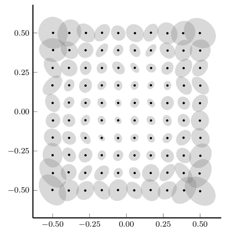
\(\color{red}{\varepsilon_{ij}} \sim N(0, |\|x_i\|^2 - \|x_j\|^2|)\)
Next Steps

Uncertainty quantification for manifold learning

Missing data and robustness

  • CMDS is known to be sensitive to missing data and/or outliers
    • We study the stability of CMDS when missing data forms a lateration graph (Arias-Castro and Vishwanath 2025)
    • Can we develop similar statistical foundations for other algorithms using robust statistics?

Other noise models

  • We consider \(D = \color{green}{\Delta(X)}+ \color{red}{\mathcal{E}}\) for \(\color{green}{X}\in \mathbb{X}\)
    • What if \(D = \Delta(Y)\) for \(Y = XR\) where \(R \in \mathbb{R}^{p \times P}\) is a random embedding matrix?

References

Arias-Castro, Ery, and Siddharth Vishwanath. 2025. “Stability of Sequential Lateration and of Stress Minimization in the Presence of Noise.” SIAM Journal on Mathematics of Data Science 7 (3): 1077–97.
Gower, John C. 1966. “Some Distance Properties of Latent Root and Vector Methods Used in Multivariate Analysis.” Biometrika 53 (3-4): 325–38.
Hall, Peter. 1979. “On the Rate of Convergence of Normal Extremes.” Journal of Applied Probability 16 (2): 433–39.
Hall, Peter. 2013. The Bootstrap and Edgeworth Expansion. Springer Science & Business Media.
Lewis, Jeffrey B, Keith Poole, Howard Rosenthal, Adam Boche, Aaron Rudkin, and Luke Sonnet. 2019. “Voteview: Congressional Roll-Call Votes Database.” See Https://Voteview. Com/(accessed 27 July 2018).
Li, Gongkai, Minh Tang, Nicolas Charon, and Carey Priebe. 2020. “Central Limit Theorems for Classical Multidimensional Scaling.” Electronic Journal of Statistics 14: 2362–94.
Schoenberg, Isaac J. 1935. “Remarks to Maurice Fréchet’s Article ‘Sur La Definition Axiomatique d’une Classe d’espace Distances Vectoriellement Applicable Sur l’espace de Hilbert’.” Annals of Mathematics 36 (3): 724–32.
Tao, Terence, and Van Vu. 2010. “Random Matrices: Localization of the Eigenvalues and the Necessity of Four Moments.” arXiv Preprint arXiv:1005.2901.
Tenenbaum, Joshua B, Vin de Silva, and John C Langford. 2000. “A Global Geometric Framework for Nonlinear Dimensionality Reduction.” Science 290 (5500): 2319–23.
Torgerson, Warren S. 1952. “Multidimensional Scaling: I. Theory and Method.” Psychometrika 17 (4): 401–19.
Vishwanath, Siddharth, and Ery Arias-Castro. 2025a. “Confidence Sets for Multidimensional Scaling.” arXiv Preprint arXiv:2510.22452.
Vishwanath, Siddharth, and Ery Arias-Castro. 2025b. “Minimax Optimality of Classical Scaling Under General Noise Conditions.” arXiv Preprint arXiv:2502.00947.
Weinberger, Kilian Q, and Lawrence K Saul. 2006. “An Introduction to Nonlinear Dimensionality Reduction by Maximum Variance Unfolding.” AAAI Conference on Artificial Intelligence 6: 1683–86.
White, Halbert. 1980. “A Heteroskedasticity-Consistent Covariance Matrix Estimator and a Direct Test for Heteroskedasticity.” Econometrica: Journal of the Econometric Society, 817–38.
Young, Gale, and Aiston S Householder. 1938. “Discussion of a Set of Points in Terms of Their Mutual Distances.” Psychometrika 3 (1): 19–22.

Thank you.

Bonus Slides

Appendix

MDS vs Dimension Reduction

Comparison MDS Dimension Reduction

Data type Pairwise dissimilarities \(\Delta\in \mathbb{R}^{n \times n}\) Feature vectors \(X \in \mathbb{R}^{n \times P}\)


Goal Find configuration \(\widehat{X}\in \mathbb{R}^{n \times p}\) such that \(\|\widehat{x}_i - \widehat{x}_j\| \approx \delta_{ij}\) Find low-dimensional representation \(\widehat{X}\in \mathbb{R}^{n \times p}\) such that \(\widehat{x}_i^{\mathsf{T}}\widehat{x}_j \approx x_i^{\mathsf{T}}x_j\)

Spectral algorithm Classical MDS (CMDS) Algorithm \[\widehat{X}= \mathop{\operatorname{arg\,min}}_{Y \in \mathbb{R}^{n \times p}} \| \Delta_c- YY^{\mathsf{T}}\|_F^2\] Principal Component Analysis (PCA) \[\widehat{X}= \mathop{\operatorname{arg\,min}}_{Y \in \mathbb{R}^{n \times p}} \| X X^{\mathsf{T}}- YY^{\mathsf{T}}\|_F^2 \]
Nonlinear methods Isomap, t-SNE, Non-metric MDS, … Kernal PCA, LLE, Laplacian Eigenmaps, …

Why CMDS works

  • In the realizable setting, there exists a latent configuration \(\color{green}{x_1, \dots, x_n} \in \mathbb{R}^p\) such that \(\color{green}{\delta_{ij} = \|x_i - x_j\|^2}\)

  • Let \(\color{green}{X} \in \mathbb{R}^{n \times p}\) be the configuration matrix

\[ \begin{aligned} \color{green}{\delta_{ij}} &= \|x_i\|^2 + \|x_j\|^2 - 2 x_i^{\mathsf{T}}x_j\\ \color{green}{\Delta} &= \text{diag}(\color{green}{X}\color{green}{X}^{\mathsf{T}})\boldsymbol{1}^{\mathsf{T}}+ \boldsymbol{1}\text{diag}(\color{green}{X}\color{green}{X}^{\mathsf{T}})^{\mathsf{T}}- 2 \color{green}{X}\color{green}{X}^{\mathsf{T}} \end{aligned} \]

\(\color{green}{\Delta_c} = -\frac{1}{2}\color{magenta}{H} \color{green}{\Delta} \color{magenta}{H} = (\color{magenta}{H}\color{green}{X})(\color{magenta}{H}\color{green}{X})^{\mathsf{T}}\)

for \(\color{magenta}{H} = I - (1/n)\boldsymbol{1}\boldsymbol{1}^{\mathsf{T}}\). The rank-\(p\) spectral decomposition of \(\Delta_c\) recovers \(\color{magenta}{H}\color{green}{X}\) (up to an orthogonal transformation):

\[ \Delta_c= (\color{magenta}{H}\color{green}{X})(\color{magenta}{H}\color{green}{X})^{\mathsf{T}}= \color{magenta}{Q}({\widehat{U}}\widehat{\Lambda }{\widehat{U}}^{\mathsf{T}})\color{magenta}{Q}^{\mathsf{T}} \]

So the CMDS embedding \(\widehat{X}= (\color{magenta}{H}\color{green}{X})\color{magenta}{Q}^{\mathsf{T}}= \color{magenta}{g}(\color{green}{X})\) recovers \(\color{green}{X}\) up to a rigid transformation \(\color{magenta}{g} \in \mathcal{G}\)

Without loss of generality, we can assume that the configuration \(X\) is centered, i.e., \(HX= X\).

Statistical Estimation and difficulties

  • Model:

    \(D = \color{green}{\Delta(X)}+ \color{red}{\mathcal{E}}\) where \(\color{red}{\mathcal{E}}= (\color{red}{\varepsilon_{ij}}) \in \mathbb{R}^{n \times n}\) is a symmetric and hollow \(n \times n\) random matrix

  • Parameters:

    \(\color{green}{X}\in \mathbb{R}^{n \times p}\) (configuration matrix underlying \(\color{green}{\Delta}\)) which consists of \(np\) unknown parameters!

As \(n \uparrow\)   then   \(\#\)parameters = \(np\!\uparrow\) too!

  • Observations:

    We have a total of \(N = \binom{n}{2}\) observations \(\big\{\delta_{ij}: i < j\big\}\)

Under the hood - I: Procrustes alignment

For each reconstruction error \(\ell_{\text{RMSE}}, \ell_2\) and \(\ell_{_{2\to\infty}}\), we have a different choice of the optimal \(g \in \mathcal{G}\)

\(\ell(\widehat{X},\color{green}{X})\) \(\displaystyle\widehat{g} = \mathop{\operatorname{arg\,min}}_{g \in \mathcal{G}} \| g(\widehat{X}) -\color{green}{X}\|_{\dagger}\)
\(\ell_{\text{RMSE}}\) \(\displaystyle\widehat{g} = \mathop{\operatorname{arg\,min}}_{g \in \mathcal{G}}\|g(\widehat{X}) - \color{green}{X}\|_F\)
\(\ell_{_{2\to\infty}}\) \(\displaystyle\widehat{g} = \mathop{\operatorname{arg\,min}}_{g \in \mathcal{G}}\|g(\widehat{X}) - \color{green}{X}\|_{_{2\to\infty}}\)


Orthogonal Procrustes Problem. For \(\color{green}{X}, Y \in \mathbb{R}^{n \times p}\) the solution to \(\color{magenta}{\color{magenta}{\widehat{g}}= \mathop{\operatorname{arg\,min}}_{g \in \mathcal{G}}\|g(Y) - \color{green}{X}\|_F}^2\) is: \[ \color{magenta}{\widehat{g}}(v) = Ov + \mu \] where \(\mu = (\overline{x} - O\overline{y})\) and \(O \in \mathcal{O}(p)\) is given by \(O = W_1W_2^{\mathsf{T}}\) where \[ W_1 S W_2^{\mathsf{T}}= \text{svd}(Y^{\mathsf{T}}\color{green}{X}) \]

Under the hood - I: Procrustes alignment

All the upper bounds are proved using \(\color{magenta}{\widehat{g}}\) obtained from the orthogonal Procrustes solution, e.g., \[ \begin{aligned} \ell_{_{2\to\infty}}(\widehat{X},\color{green}{X}) &= \min_{g \in \mathcal{G}}\|g(\widehat{X}) - \color{green}{X}\|_{_{2\to\infty}} \\ &\color{magenta}{\le} \bbox[yellow]{\| \color{magenta}{\widehat{g}}(\widehat{X}) -\color{green}{X}\|_{_{2\to\infty}} \;\lesssim\; \overline{c}({\kappa, \varpi})\cdot \sigma\sqrt{\frac{\log{n}}{n}}} \end{aligned} \]


Orthogonal Procrustes Problem. For \(\color{green}{X}, Y \in \mathbb{R}^{n \times p}\) the solution to \(\color{magenta}{\color{magenta}{\widehat{g}}= \mathop{\operatorname{arg\,min}}_{g \in \mathcal{G}}\|g(Y) - \color{green}{X}\|_F}\) is: \[ \color{magenta}{\widehat{g}}(v) = Ov + \mu \] where \(\mu = (\overline{x} - O\overline{y})\) and \(O \in \mathcal{O}(p)\) is given by \(O = W_1W_2^{\mathsf{T}}\) where \[ W_1 S W_2^{\mathsf{T}}= \text{svd}(Y^{\mathsf{T}}\color{green}{X}) \]

Under the hood - II: Fuk-Nagaev-Type concentration

Let \(\mathcal{E}= (\varepsilon_{ij})\) be an \(n \times n\) random matrix where each row \(\varepsilon_{i, *}\) consists of independent entries. Let \(X \in \mathbb{R}^{n \times p}\) be fixed.

Bernstein-Type Concentration.   If \(\max_{i,j}|{\varepsilon_{i,j}|} \le K\) a.s., then with probability greater than \(1 - O({e^{-t}})\), \[ \|\mathcal{E}X\|_{2\to\infty}\lesssim \sigma_2 \sqrt{n (t + \log{p})} + K (t + \log{p}) \]


Fuk-Nagaev-Type Concentration (Vishwanath and Arias-Castro 2025b)   Suppose \(\max_{i,j}\|{\varepsilon_{i,j}\|_{L^q}} \le \sigma\) for \(q > 4\)
Then, for all \(0 < r < \frac{(q-4)}{2}\), with probability greater than \(1 - O({e^{-t}} + {n^{-r}})\), \[ \|\mathcal{E}X\|_{2\to\infty}\lesssim \sigma_2 \sqrt{n (t + \log{p})} + \sigma n^{(r+2)/q} (t + \log{p}) \]

\(\sigma_2 = \max_{i,j} \|{\varepsilon_{ij}}\|_{L^2}\)
Operator norm version in the appendix

Under the hood - II: Fuk-Nagaev matrix concentration

Classical Fuk-Nagaev Inequality.

Suppose \(Z_1, \dots, Z_n\) are independent with \(\mathbb{E}(Z_i) = 0\) and \(\|Z_i\|_{L^q} \le \sigma\) for some \(q \ge 2\)

Let \(S_n = \sum_i Z_i\). For all \(0 < r < \frac{(q-2)}{2}\), with probability greater than \(1 - O({e^{-t}} + {n^{-r}})\), \[ |S_n| \lesssim {\sqrt{t \sum_i \text{Var}(Z_i)}} + {\sigma n^{(r+1)/q}} \]

Under the hood - II: Fuk-Nagaev matrix concentration

(Vishwanath and Arias-Castro 2025b, Proposition 3)

Suppose \(\mathcal{E}= (\varepsilon_{ij})\) is a symmetric random matrix with independent entries and \(\|\varepsilon_{ij}\|_{L^4} \le \sigma\) for \(q > 4\)

Then, for all \(0 < r < \frac{(q-4)}{2}\), with probability greater than \(1 - O({e^{-t}} + {n^{-r}})\), \[ \begin{aligned} \|\mathcal{E}\|_2 \lesssim \underbrace{\max_{i}\sqrt{\sum_{j} \text{Var}(\varepsilon_{ij})} + \sigma n^{(r+2)/q}\sqrt{t + \log{n}}}_{\text{sub-Gaussian + polynomial tail}} \end{aligned} \]

Under the hood - III: Four moments are necessary


Metric CMDS Upper Bound Minimax Lower Bound

\[\ell_{\text{RMSE}}\] \(\displaystyle\frac{\sigma\kappa}{\sqrt{n}}\) \(\displaystyle\frac{\sigma\kappa}{\sqrt{n}}\)

\(\ell_{_{2\to\infty}}\) \(\displaystyle\overline{c}({\kappa, \varpi})\cdot \sigma\sqrt{\frac{\log{n}}{n}}\) \(\displaystyle\underline{c}({\kappa, \varpi})\cdot \sigma\sqrt{\frac{\log{n}}{n}}\)


  • \(q > 4\) moments is necessary for consistency (c.f., Tao and Vu 2010)
  • where \(\overline{c}({\kappa, \varpi}) = \kappa^2(\kappa + \varpi)\) and \(\underline{c}({\kappa, \varpi}) = \kappa(1+\kappa\varpi)^{-1}\)

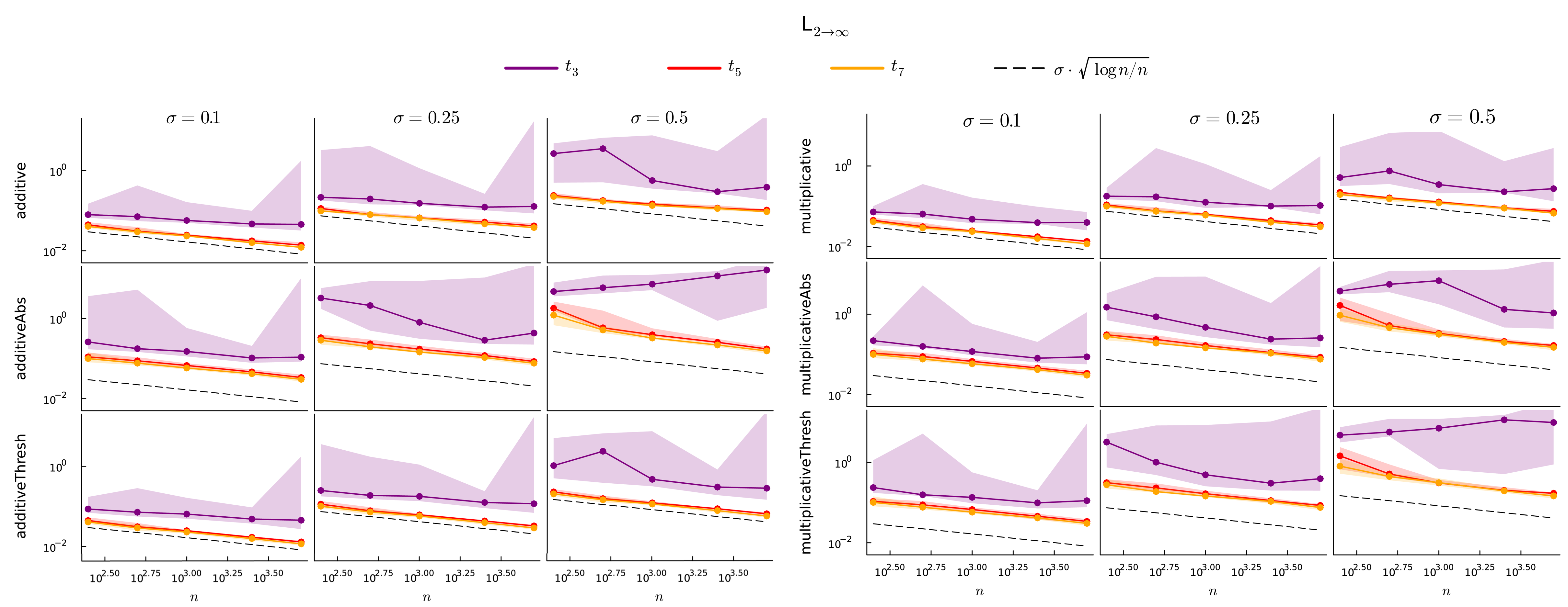
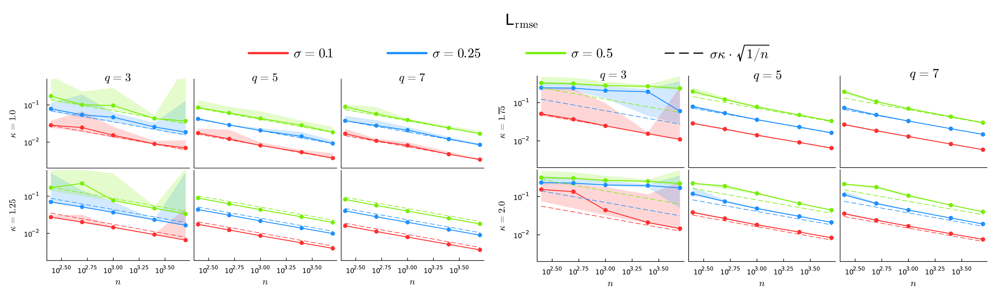
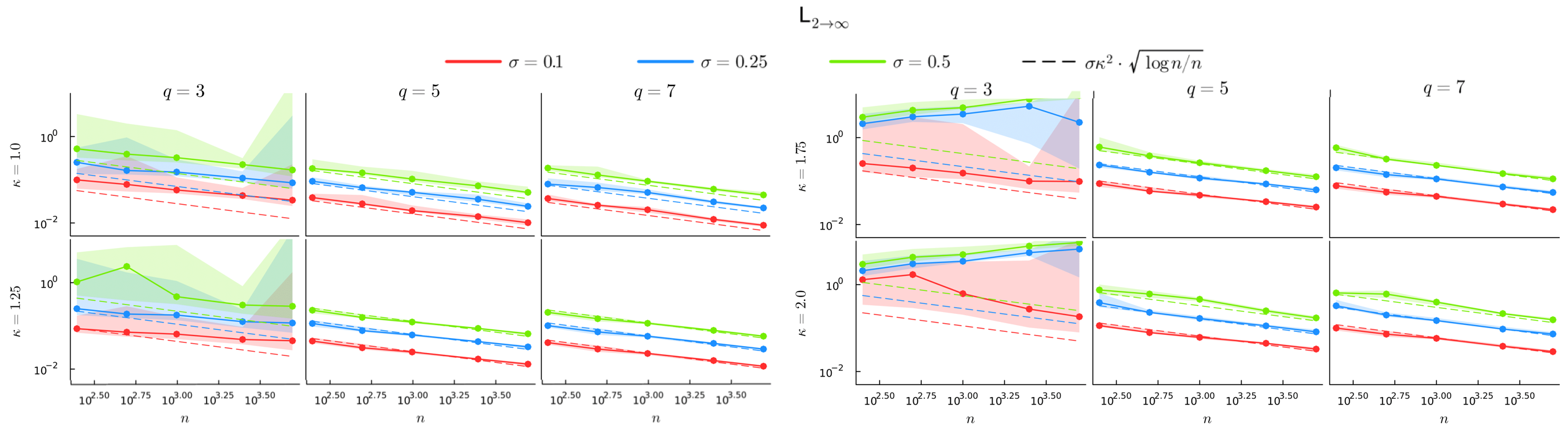
Appendix: Comparison

  • \(\color{green}{X}\in \mathbb{R}^{n \times p}\) are chosen from an ellipsoid with condition number \(\kappa^2\)
  • \(D = \color{green}{\Delta(X)}+ \color{red}{\mathcal{E}}\) under different noise models with \(\color{red}{\varepsilon_{ij}} \sim t_q\) entries
Appendix: Comparison
Slightly stronger assumptions

\(\color{red}{\mathcal{E}}= (\color{red}{\varepsilon_{ij}})\) is a random symmetric hollow matrix with:

  1. Independence: \(\hspace{1em}\) \((\color{red}{\varepsilon_{ij}})\) are independent for \(i < j\) with \(\mathbb{E}(\color{red}{\varepsilon_{ij}}) = 0\) and \(\text{Var}(\color{red}{\varepsilon_{ij}}) = \sigma_{ij}^2\)
  2. sub-Exponential tails: \(\hspace{1em}\) \(\displaystyle\max_{i < j}\|\color{red}{\varepsilon_{ij}}\|_{{\psi_1}} \le \overline{\sigma}\)
  3. Non-degenerate* \(\hspace{1.5em}\) For \(\underline{\sigma}> 0\), \(\hspace{1em}\) \(\displaystyle\min_{i < j}\sigma_{ij} \ge \underline{\sigma}\)

Local covariance information

  • \(\|{\widehat{X}- \color{magenta}{\widehat{g}}(X)}\|_{2\to\infty}\) leads to uniformly spherical sets

\(\displaystyle\Big\{Y \in \mathbb{R}^{n \times p}: \|{\widehat{X}- Y}\|_{2\to\infty} \le r \Big\} = \prod_{i=1}^n B(\widehat{x}_i, r)\)

  • For \(\mathcal{E}= (\varepsilon_{ij})\) let \(\Sigma_i = \text{diag}( \sigma_{i1}^2, \dots, \sigma_{in}^2 )\). Then,

\(\displaystyle\Omega_i := \frac{n}{4} (\color{green}{X}^{\mathsf{T}}\color{green}{X})^{-1}\color{green}{X}^{\mathsf{T}}\Sigma_i\color{green}{X}(\color{green}{X}^{\mathsf{T}}\color{green}{X})^{-1} \in \mathbb{R}^{p \times p}\)

captures the local covariance structure at each \(\widehat{x}_i \in \mathbb{R}^p\)

  • Let \(E = (e_{ij}) = D - \Delta(\widehat{X})\) be the matrix of residuals. The plug-in estimator* for \(\Omega_i\) is

\(\displaystyle\widehat{\Omega}_i := \frac{n}{4} (\widehat{X}^{\mathsf{T}}\widehat{X})^{-1} \widehat{X}^{\mathsf{T}}\widehat{\Sigma}_i \widehat{X}(\widehat{X}^{\mathsf{T}}\widehat{X})^{-1} \in \mathbb{R}^{p \times p}\)

where \(\widehat{\Sigma}_i = \text{diag}( e_{i1}^2, \dots, e_{in}^2 )\)

This is the analogue of White’s correction for heteroscedasticity (White 1980)

Local covariance information

  • \(\|{\color{magenta}{\widehat{g}}(\widehat{X}) - X}\|_{2\to\infty}\) leads to uniformly spherical sets.

\(\displaystyle\Big\{X \in \mathbb{R}^{n \times p}: \|{\widehat{X}- \color{magenta}{\widehat{g}}(X)}\|_{2\to\infty} \le r \Big\} = \prod_{i=1}^n B(\widehat{x}_i, r)\)

  • Consider the statistic \(\widehat{T}_n\) given by

\[ \widehat T_n := \max_{i \in [n]} \sqrt{n}\|\widehat{\Omega}_i^{-1/2}\left(x_i - \color{magenta}{\widehat{g}}(\widehat{x}_i)\right)\|. \]

  • \(\widehat T_n\) leads to locally ellipsoidal sets

\(\displaystyle\Big\{X \in \mathbb{R}^{n \times p}: \widehat T_n \le r \Big\} = \prod_{i=1}^n \mathscr{E}\big(\widehat{x}_i,\; \widehat{\Omega}_i,\; r\big)\)

where \(\mathscr{E}(z, \Omega, r) := \{ x \in \mathbb{R}^p : (x - z)^{\mathsf{T}}\Omega^{-1} (x - z) \le r^2 \}\)

Beyond Gaussian Multiplier Bootstrap

\(\color{green}{X}\in \mathbb{R}^{350 \times 2}\) is the location of the \(350\) largest US cities and \(\log d_{ij} = \color{green}{\log\delta_{ij}} + \color{red}{\varepsilon_{ij}}\) where \(\color{red}{\varepsilon_{ij}} \sim N(0, \sigma^2 )\)

  1. Gaussian multipliers \(r_{ij} \sim N(0, 1)\)
  2. Rademacher multipliers \(r_{ij} \sim \text{Rademacher}(\pm 1)\)
  3. Uniform multipliers \(r_{ij} \sim \text{Unif}([- \sqrt{3}, \sqrt{3}])\)


Nominal level \(\rightarrow\) 0.999 0.99 0.975 0.95 0.925 0.9 0.85 0.8 0.75
Gaussian 0.998 0.992 0.983 0.954 0.932 0.902 0.851 0.789 0.707
Rademacher 0.997 0.988 0.980 0.951 0.924 0.895 0.825 0.738 0.628
Uniform 0.997 0.991 0.983 0.953 0.930 0.897 0.837 0.750 0.659
Empirical 1.000 1.000 1.000 1.000 0.997 0.994 0.994 0.953 0.983
Gumbel 0.939 0.847 0.772 0.690 0.630 0.580 0.508 0.423 0.356